sphinterpolate

sphinterpolate(cmd0::String="", arg1=nothing, kwargs...)

keywords: GMT, Julia, spherical grid interpolation

Spherical gridding in tension of data on a sphere.

Description

Reads lon, lat, z from file or table and performs a Delaunay triangulation to set up a spherical interpolation in tension. The final grid is saved to the specified file. Several options may be used to affect the outcome, such as choosing local versus global gradient estimation or optimize the tension selection to satisfy one of four criteria.

Required Arguments

• table
  One or more data tables holding a number of data columns.

• I or inc or increment or spacing : – inc=x_inc | inc=(xinc, yinc) | inc="xinc[+e|n][/yinc[+e|n]]"
  Specify the grid increments or the block sizes. More at spacing

• R or region or limits : – limits=(xmin, xmax, ymin, ymax) | limits=(BB=(xmin, xmax, ymin, ymax),) | limits=(LLUR=(xmin, xmax, ymin, ymax),units="unit") | ...more
  Specify the region of interest. More at limits. For perspective view view, optionally add zmin,zmax. This option may be used to indicate the range used for the 3-D axes. You may ask for a larger w/e/s/n region to have more room between the image and the axes.

Optional Arguments

• D or skipdup : skipdup=true | skipdup=:east
  Skip duplicate points since the spherical gridding algorithm cannot handle them. [Default assumes there are no duplicates, except possibly at the poles]. Append a repeating longitude (east) to skip records with that longitude instead of the full (slow) search for duplicates.

• Q or tension : – tension=mode
  Specify one of four ways to calculate tension factors to preserve local shape properties or satisfy arc constraints [Default is no tension]. Use:

  • tension=:p for piecewise linear interpolation; no tension is applied.

  • tension=:l for local Smooth interpolation with local gradient estimates.

  • tension=:g for global Smooth interpolation with global gradient estimates. You may optionally append N/M/U (e.g. (invented) tension="g1/2/3), where N is the number of iterations used to converge at solutions for gradients when variable tensions are selected (e.g., var_tension only) [3], M is the number of Gauss-Seidel iterations used when determining the global gradients [10], and U is the maximum change in a gradient at the last iteration [0.01].

  • tension=:s for smoothing. Optionally append E/U/N [/0/0/3], where E is Expected squared error in a typical (scaled) data value, and U is Upper bound on weighted sum of squares of deviations from data. Here, N is the number of iterations used to converge at solutions for gradients when variable tensions are selected (e.g., var_tension only) [3]

• G or save or outgrid or outfile : – outgrid=[=ID][+ddivisor][+ninvalid][+ooffset|a][+sscale|a][:driver[dataType][+coptions]]
  Give the name of the output grid file. Optionally, append =ID for writing a specific file format (See full description). The following modifiers are supported:

  • +d - Divide data values by given divisor [Default is 1].

  • +n - Replace data values matching invalid with a NaN.

  • +o - Offset data values by the given offset, or append a for automatic range offset to preserve precision for integer grids [Default is 0].

  • +s - Scale data values by the given scale, or append a for automatic scaling to preserve precision for integer grids [Default is 1].

Note1: Any offset is added before any scaling. +sa also sets +oa (unless overridden). To write specific formats via GDAL, use =gd and supply driver (and optionally dataType) and/or one or more concatenated GDAL -co options using +c. See the “Writing grids and images” cookbook section for more details.

Note2: This is optional and to be used only when saving the result directly on disk. Otherwise, just use the G = modulename(...) form.

• T or var_tension : var_tension=true
  Use variable tension.

• V or verbose : – verbose=true | verbose=level
  Select verbosity level. More at verbose

• Z or scale : – scale=true
  Before interpolation, scale data by the maximum data range [no scaling].

• bi or binary_in : – binary_in=??
  Select native binary format for primary table input. More at

• di or nodata_in : – nodata_in=??
  Substitute specific values with NaN. More at

• e or pattern : – pattern=??
  Only accept ASCII data records that contain the specified pattern. More at

• h or header : – header=??
  Specify that input and/or output file(s) have n header records. More at

• i or incol or incols : – incol=col_num | incol="opts"
  Select input columns and transformations (0 is first column, t is trailing text, append word to read one word only). More at incol

• q or inrows : – inrows=??
  Select specific data rows to be read and/or written. More at

• r or reg or registration : – reg=:p | reg=:g
  Select gridline or pixel node registration. Used only when output is a grid. More at

• s or skiprows or skip_NaN : – skip_NaN=true | skip_NaN="<cols[+a][+r]>"
  Suppress output of data records whose z-value(s) equal NaN. More at

• yx : – yx=true
  Swap 1st and 2nd column on input and/or output. More at

Examples

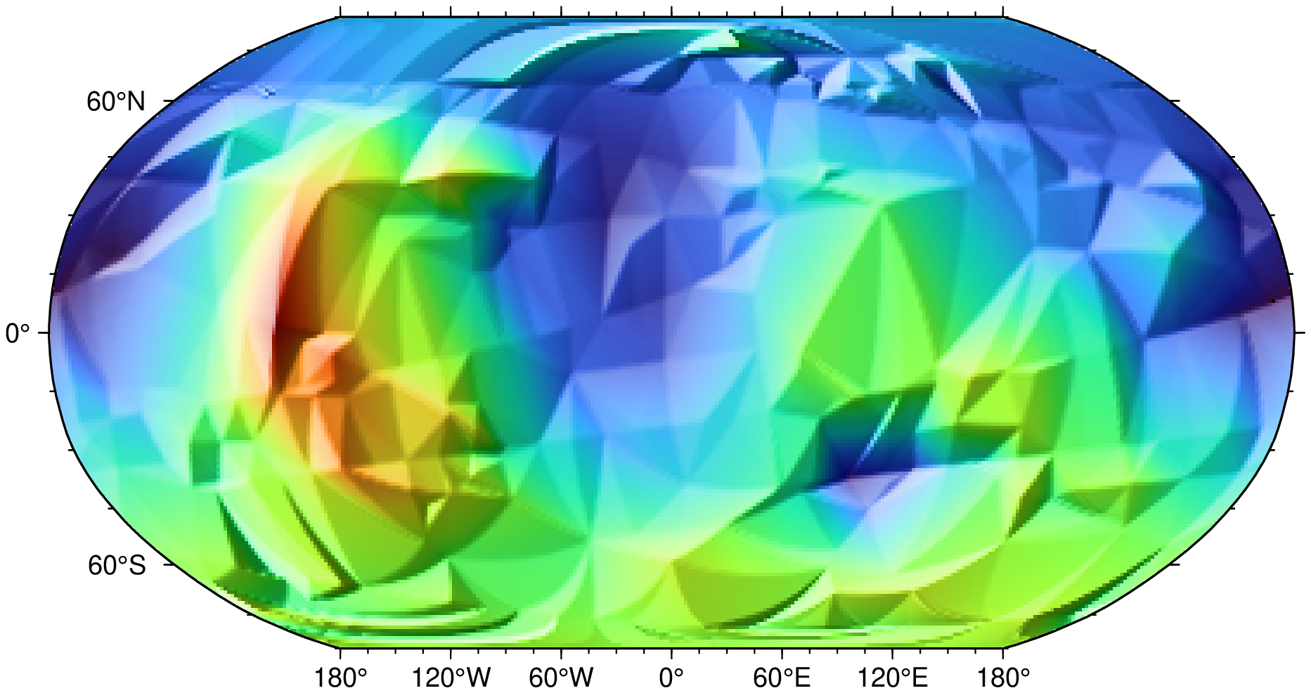
To interpolate data from the remote file mars370d.txt using the piecewise method for a 1x1 global grid, then plot it, try:

using GMT
G = sphinterpolate("@mars370d.txt", region=:global, inc=1, tension=:p)
imshow(G, proj=:guess, shade=true)

To interpolate the points in the file testdata.txt on a global 1x1 degree grid with no tension, use:

G = sphinterpolate("testdata.txt", region=:global, inc=1)

Notes

The STRIPACK algorithm and implementation expect that there are no duplicate points in the input. It is best that the user ensures that this is the case. GMT has tools, such as blockmean and others, to combine close points into single entries. Also, sphinterpolate has a skipdup option to determine and exclude duplicates, but it is a very brute-force yet exact comparison that is very slow for large data sets. A much quicker check involves appending a specific repeating longitude value. Detection of duplicates in the STRIPACK library will exit the module.

See Also

greenspline, nearneighbor, sphdistance, sphtriangulate, surface, triangulate

References

Renka, R, J., 1997, Algorithm 772: STRIPACK: Delaunay Triangulation and Voronoi Diagram on the Surface of a Sphere, AMC Trans. Math. Software, 23\ (3), 416-434.

Renka, R, J,, 1997, Algorithm 773: SSRFPACK: Interpolation of scattered data on the Surface of a Sphere with a surface under tension, AMC Trans. Math. Software, 23\ (3), 435-442.