vband
vband(mat::Matrix; region=(...), width=false,  percent=false, fill=nothing, fillalpha=nothing)

hband(mat::Matrix; region=(...), height=false, percent=false, fill=nothing, fillalpha=nothing)
keywords: GMT, Julia, plot
Reads a MxN array where 2 <= N <= 4 and plot a vertical (vband or vspan) or horizontal (hband or hspan) bands across the xy plot. If N == 2 the bands are plotted from ymin to ymax (vband) and from xmin to xmax (hband). The optional 1 or 2 extra columns control the begin/end of each band (see examples). The third (optional) column specifies the base of a vertical band or the left of the horizontal one. Use a NaN to indicate that base|left = y|x_min. The 4rth column controls the top of vertical bands or the right of the horizontals. Also here a NaN means top|right = y|x_max.
The bands width (or height in hband) are controlled by two alternative mechanisms. By default the input mat array has rows with x1 x2 (data) coordinates for the start and end of each vband and y1 y2 for each hband. But alternatively we may specify width=true (for vbands) or percent=true in which case the second column is interpreted as the band width (or height in hband) or the percentage of the plot's width (height) in data units.
A small annoyance in using these functions in a first call is that we must specify the plot limits. To minimize this constrain, we can call them from with a plot call as a nested call (see example at the bottom). But even here we have a lower order annoyance. When called nested in plot the bands will be plotted over the lines/symbols and not under as it would be desirable. Mechanics of GMT make this difficult to achieve.
For syntax compatibility with other Julia plotting packages vband and hband have aliases vspan and hspan.
Parameters
B or axes or frame
Set map boundary frame and axes attributes. Default is to draw and annotate left, bottom and vertical axes and just draw left and top axes. More at frame
J or proj or projection : – proj=<parameters>
Select map projection. More at proj
R or region or limits : – limits=(xmin, xmax, ymin, ymax) | limits=(BB=(xmin, xmax, ymin, ymax),) | limits=(LLUR=(xmin, xmax, ymin, ymax),units="unit") | ...more
Specify the region of interest. More at limits. For perspective view view, optionally add zmin,zmax. This option may be used to indicate the range used for the 3-D axes. You may ask for a larger w/e/s/n region to have more room between the image and the axes.
fill or color
Select color or pattern for filling of symbols [Default is lightblue]. It can take the form of a string, a vector or a tuple of colors. See Setting color for extend color selection (including color map generation). When more than one band is requested the bands colors are assigned by cycling through the colors given in this option. This means that a 3 bands and afill=[:red, :blue]will plot first and third band in red and second in blue.
Optionally the fill can be done with patterns (which includes the possibility of using images).
fillalpha or alpha or transparency : – alpha=0.5 | alpha=(50, 75)
Control the transparency level. Numbers can be floats <= 1.0 or integers in 0-100 range. Default is 75. It can take the form of a number, a vector or a tuple of numbers. When more than one band is requested the bands transparencies are assigned by cycling through the values given in this option. This means that the number of bands and of transparencies may be different.
figname or savefig or name : – figname=
name.png
Save the figure with thefigname=name.extwhereextchooses the figure image format.
Examples
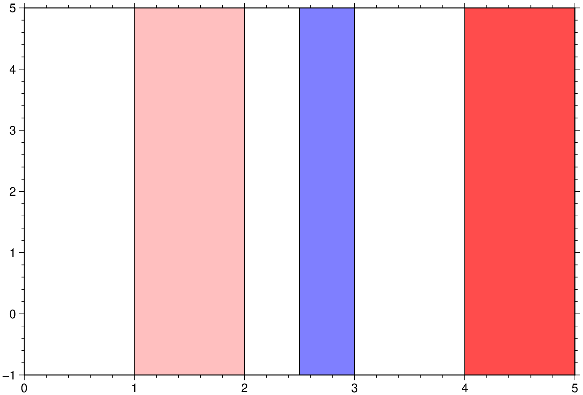
A vertical bands with 2 colors and 3 transparencies
using GMT
vband([1 2; 2.5 3; 4 5], fill=(:red, :blue), alpha=(0.75, 0.5, 0.3), region=(0,5,-1,5), show=true)
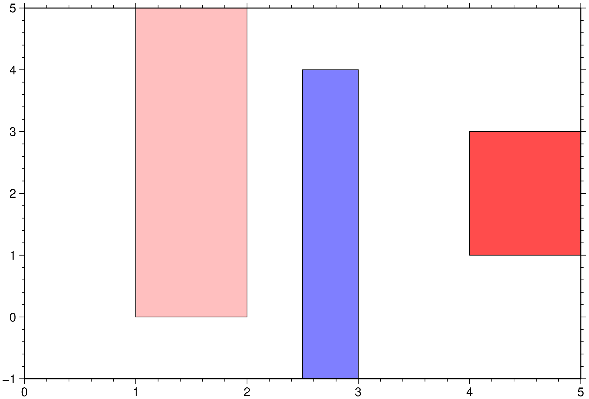
Now with variable heights.
using GMT
vband([1 2 0 NaN; 2.5 3 NaN 4; 4 5 1 3], fill=[:red, :blue], alpha=(0.75, 0.5, 0.3),
      region=(0,5,-1,5), show=true)
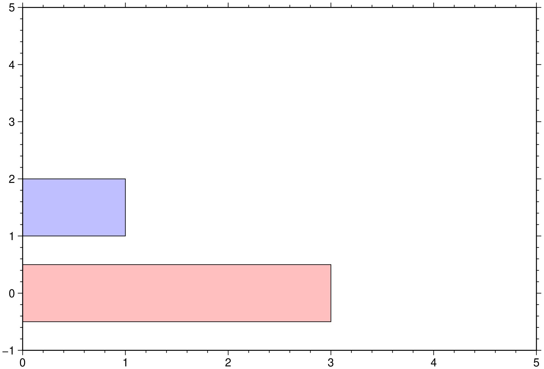
A horizontal band plot with variable lengths and colors and constant transparency.
using GMT
hband([-0.5 0.5 0 3; 1 2 1 NaN; 3 4 NaN NaN], fill=(:red, :blue, :green), region=(0,5,-1,5), show=1)
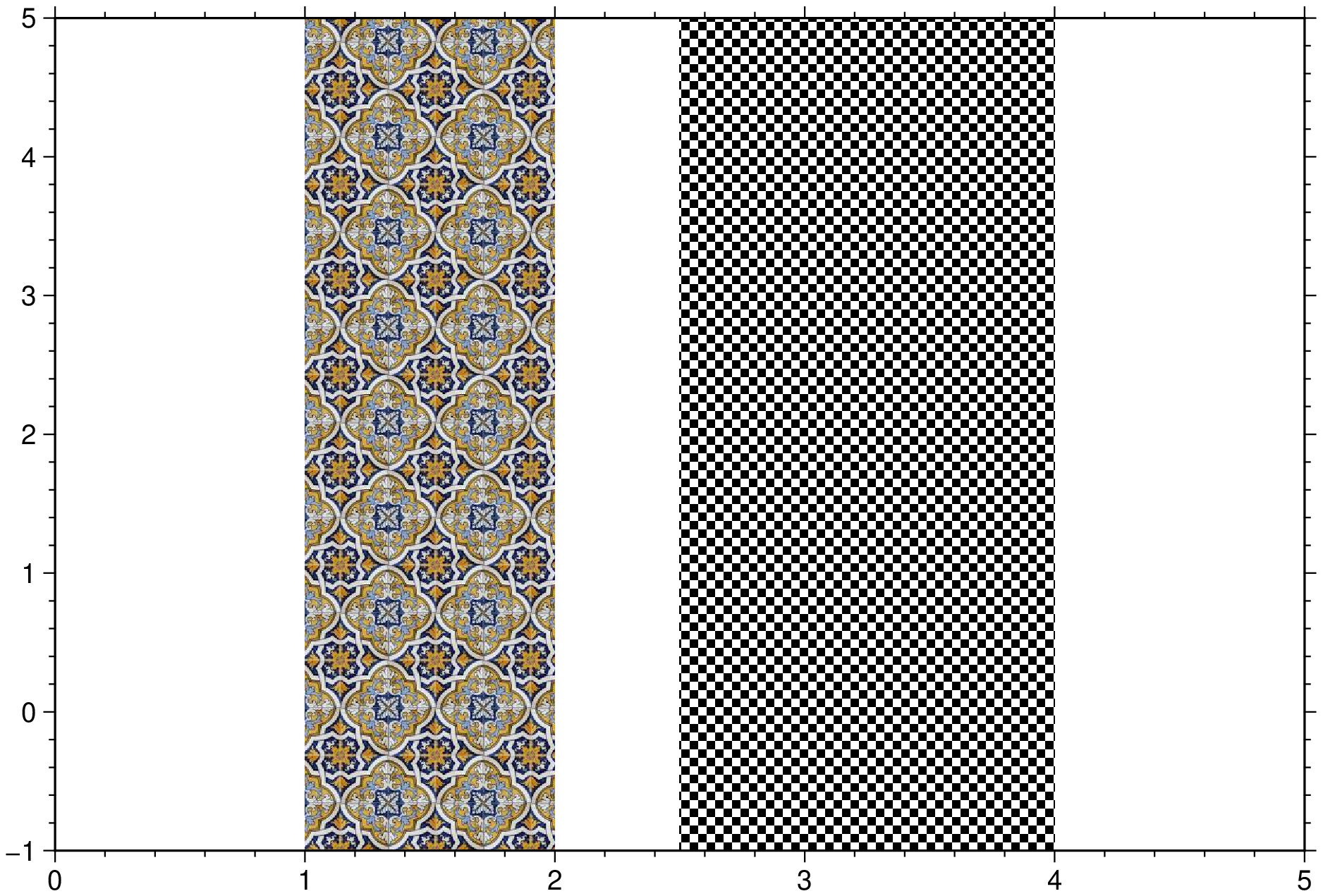
We can fill with patterns as well. And use an image as one of the patterns.
using GMT
vband([1 2; 2.5 4], fill=((pattern=GMT.TESTSDIR * "tiling2.jpg", dpi=200), (pattern=27, dpi=200)),
      region=(0,5,-1,5), show=true)
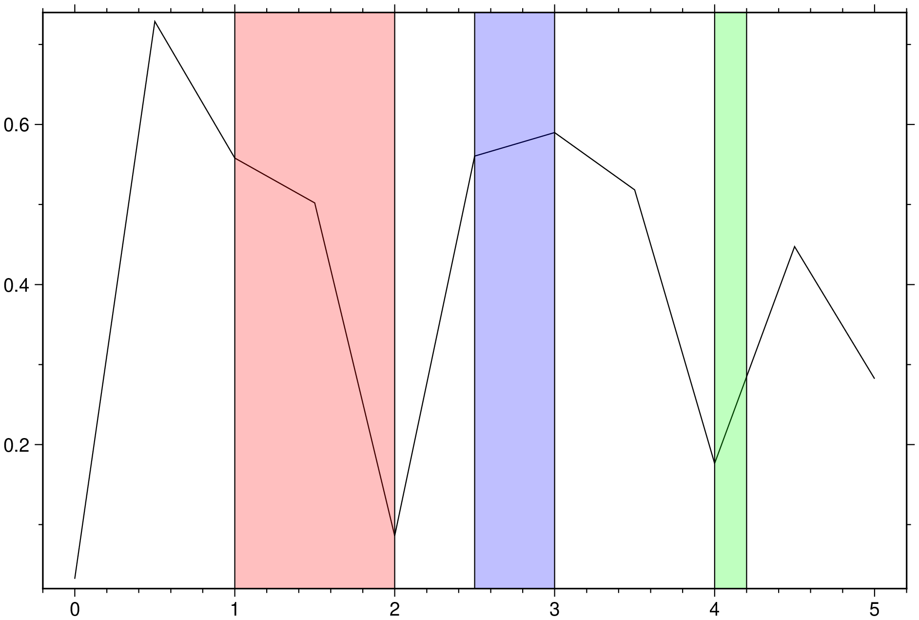
Do a nested call in which one is not forced to specify the plot limits but let it be computed from input data
using GMT
plot(0:0.5:5, rand(11), vband=(data=[1 2; 2.5 3; 4 4.2], fill=[:red, :blue, :green]), show=true)
See also
These docs were autogenerated using GMT: v1.11.0