Navigation

Ternary plots

See manual at ternary

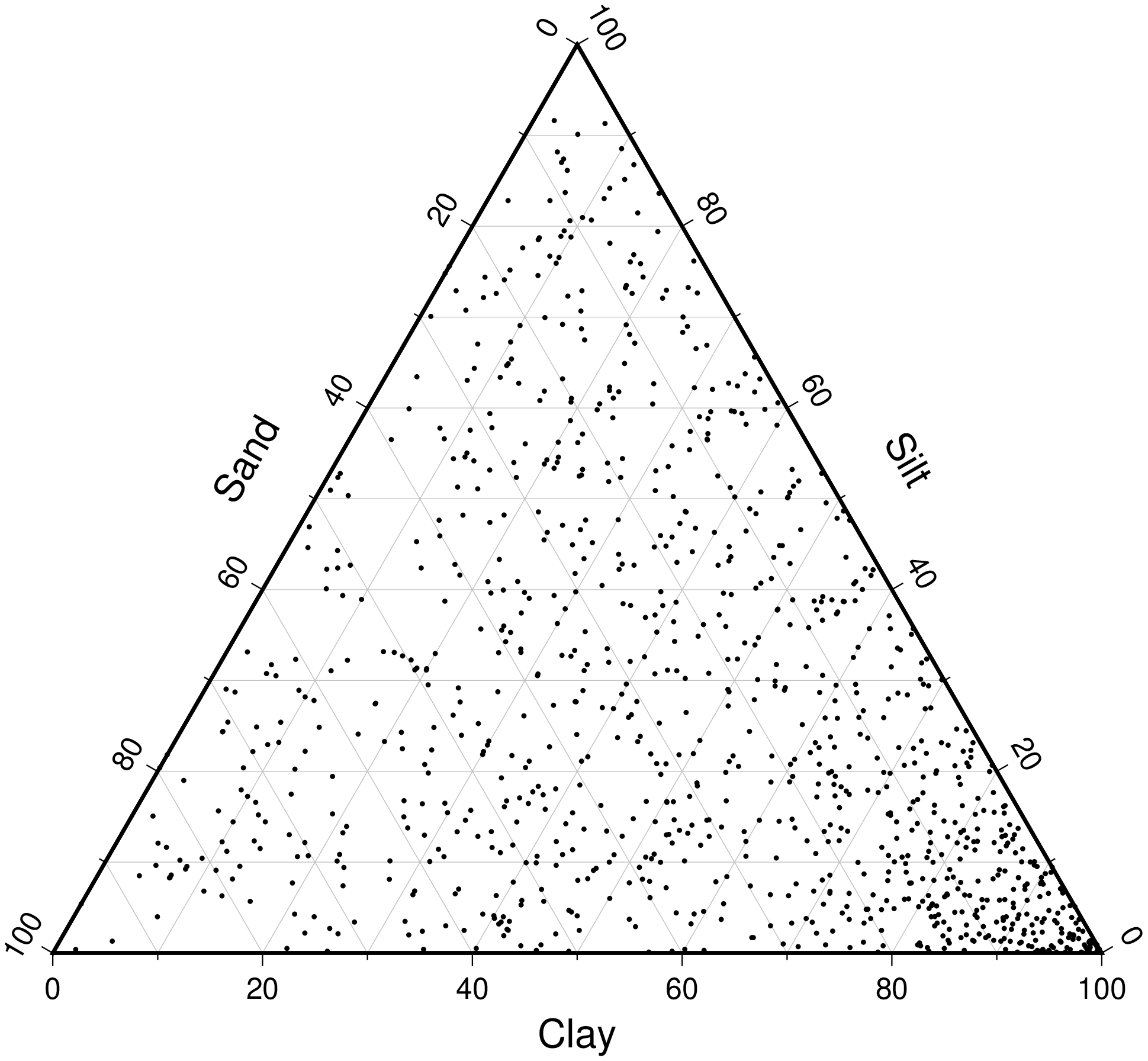
A scatter plot example

To plot points on a ternary diagram at the positions listed in the file ternary.txt (that GMT knows where to find it), with default annotations and gridline spacings, using the specified labeling, do:

using GMT
ternary("@ternary.txt", labels=("Clay","Silt","Sand"), marker=:p, show=true)

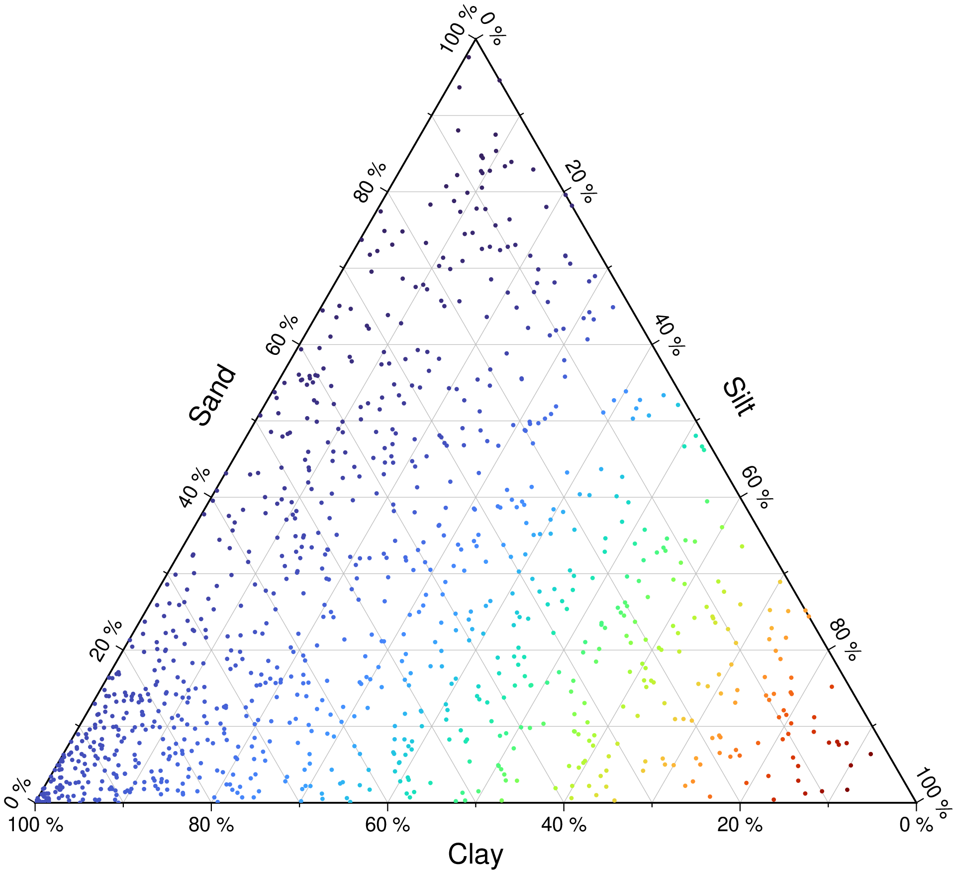
– Ok, good but a bit dull. What about coloring the points? And if I want to have the axes runing in clock-wise order? And what about adding a percentage symbol to the annotations?

Simple. First we create a colormap and to rotte the axes we use the option clockwise=true. Regarding the % sign, it requires using the frame option and that obliges to be explicit on the axes labels because we are no longer using handy defaults.

using GMT
# Make use of the knowledge that z ranges berween 0 and 71 (gmtinfo module is a friend)
C = makecpt(T=(0,71));
ternary("@ternary.txt",  marker=:p, cmap=C, clockwise=true, 
        frame=(annot=:auto, grid=:a, ticks=:a, alabel="Clay", blabel="Silt",
        clabel="Sand", suffix=" %"), show=true)

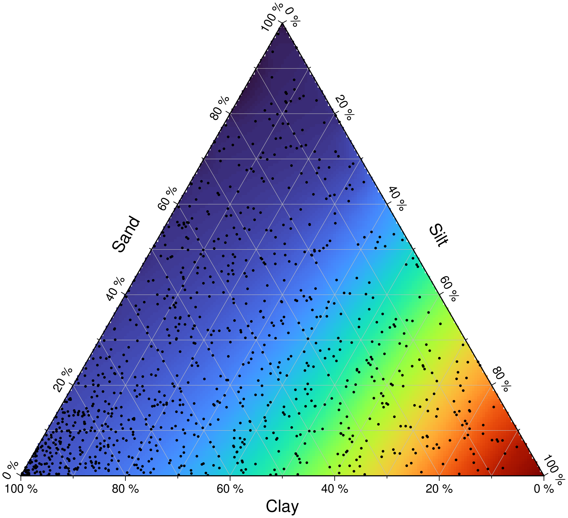
Ternary with image

Ah, much better, but now I would like to display the above data as an image.

Solution: use the image=true option. Note that we may skip the cmap option and an automatic cmap is compute for us (but one can use whatever cmap we want, just create a colormap with the wished colors)

using GMT
ternary("@ternary.txt", marker=:p, image=true, clockwise=true,
        frame=(annot=:auto, grid=:a, ticks=:a, alabel="Clay", blabel="Silt",
        clabel="Sand", suffix=" %"), show=true)

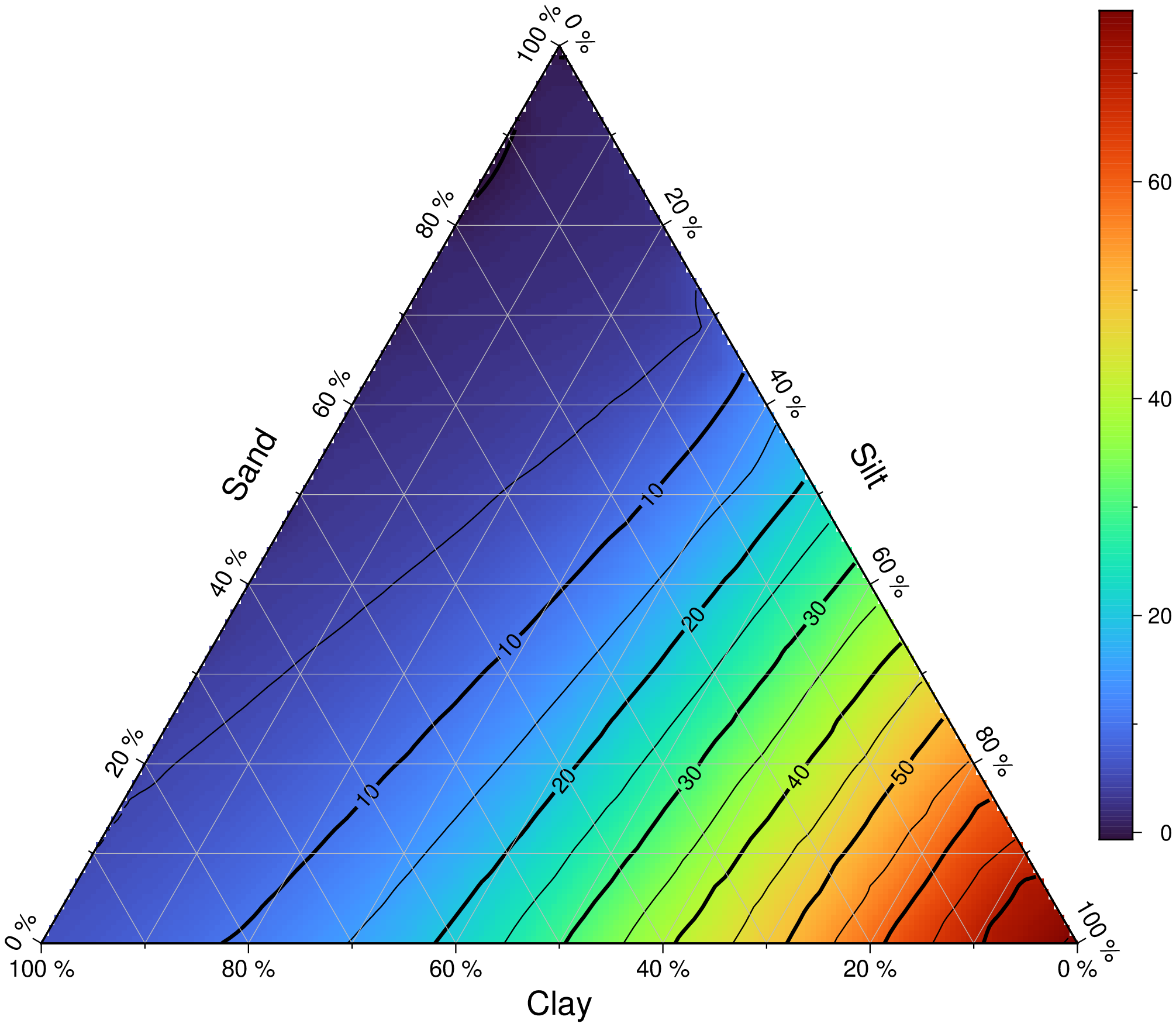
And to overlay some contours?

Add the contour option. This option works either with automatically picked parameters or under the user full control (which contours to draw and which to annotate, etc). For simplicity we could use the automatic mode (just set contour=true) but the ternary plots may have several short contour lines that would not be annotated because they are too short for the default setting. So, and for demonstration sake, we will use the explicit contour form where we set also the distance between the labels.

using GMT
ternary("@ternary.txt", clockwise=true, image=true, 
        frame=(annot=:auto, grid=:a, ticks=:a, alabel="Clay", blabel="Silt", clabel="Sand", suffix=" %"),
        contour=(annot=10, cont=5, labels=(distance=3,)),
        colorbar=true, show=true)

And we can do a contourf style plot too, but in this case only the area inside the data cloud is imaged since the method used involves a Delaunay triangulation.

using GMT
ternary("@ternary.txt", marker=:p, clockwise=true, 
        frame=(annot=:auto, grid=:a, ticks=:a, alabel="Clay", blabel="Silt", clabel="Sand", suffix=" %"),
        contourf=(annot=10, cont=5), show=true)

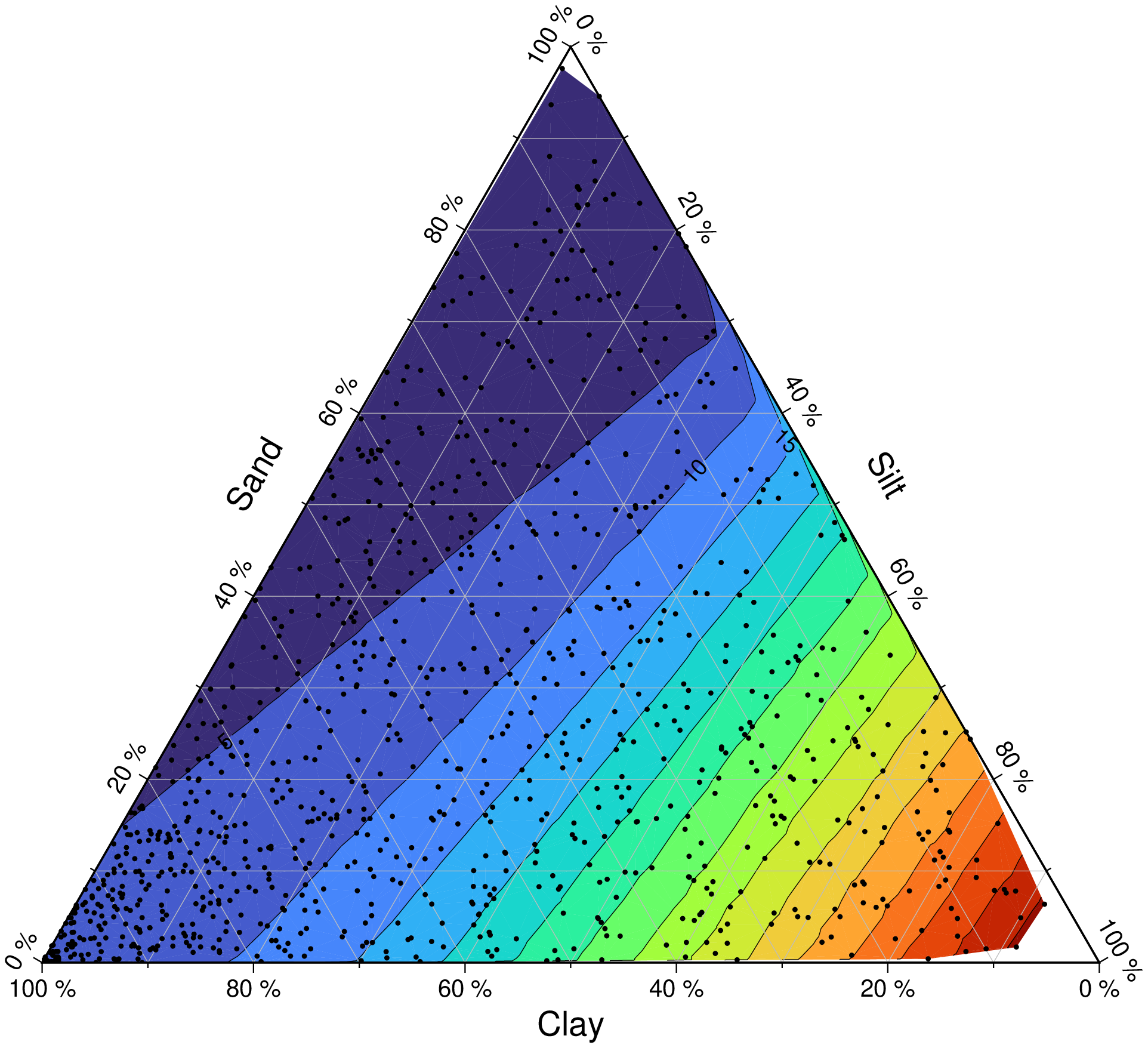
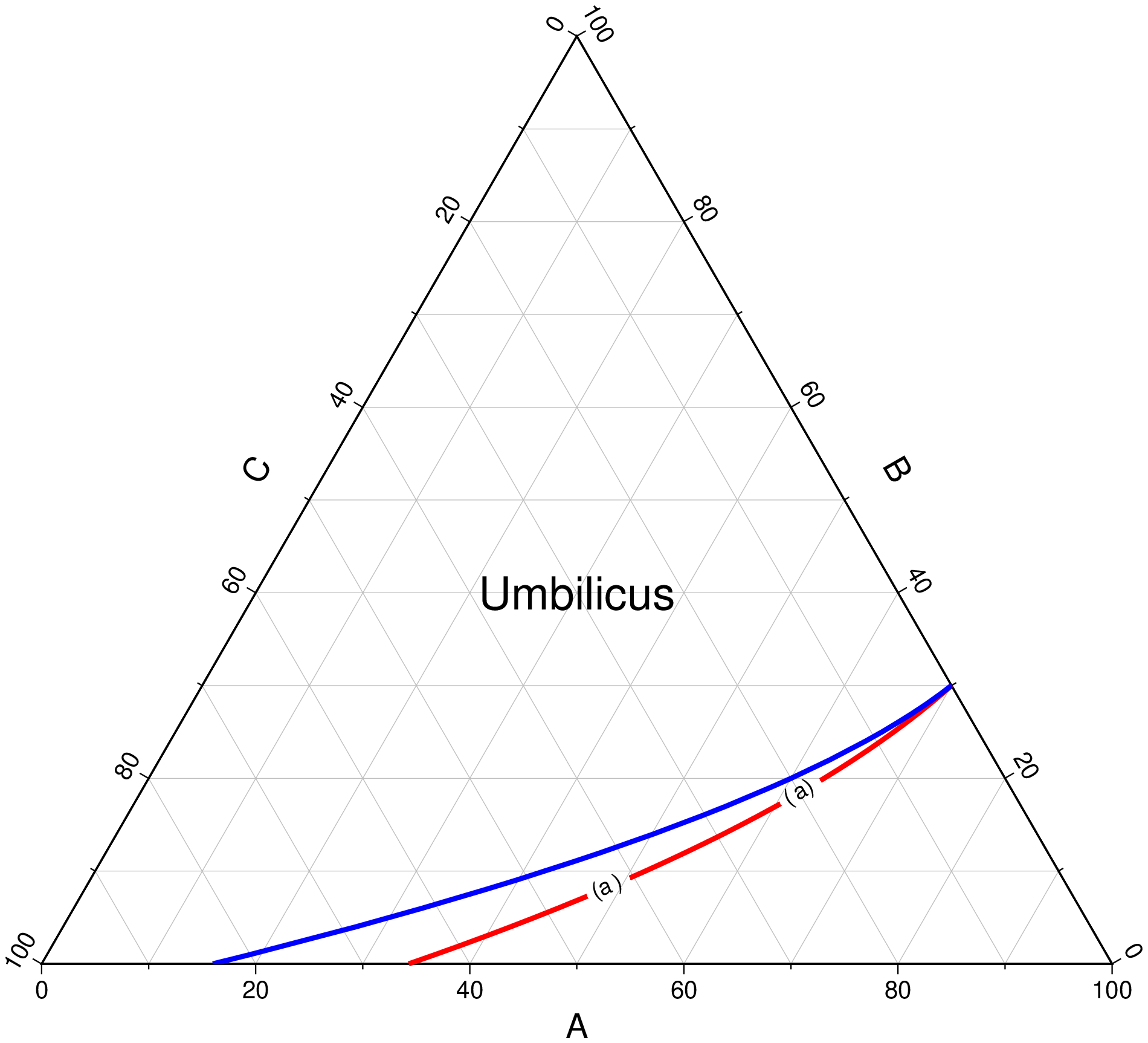
Diagram with lines and text

This example makes use of the tern2cart function that converts from ternary to cartesian coordinates. It is based on this discussion of the Julia forum.

using GMT

b = 0:0.01:0.3
c1 = (1 .- b).^3 .- 0.7^3
c2 = (1 .- 2*b).^2 .- 0.4^2

# Generate the coordinates of two lines.
t1 = tern2cart([(1 .- b .- c1) b c1])    # Note that GMT.jl function expects a Mx3 matrix
t2 = tern2cart([(1 .- b .- c2) b c2])

ternary(labels=("A", "B", "C"))

plot!(t1, lw=2, lc=:red, ls="line& (a) &")	# line style -> fancy stuff
plot!(t2, lw=2, lc=:blue)
text!(tern2cart([0.3 0.4 0.3]), text="Umbilicus", font=18, show=true)