Compute the time rate of change of an stack of SST data
Here we are going to compute the time rate of change (i.e. the temperature variation) for all points of the region of the stack obtained in the "Make a stack of L3 MODIS files" Lesson. We will do that using both the annual means, and directly from the monthly means. As we will see later both procedures will not give exactly the same result.
Open the stack of montly SST data created in "Make a stack of L3 MODIS files" Lesson
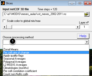
When you open the stack SST monthly file besides the display of the first layer in file, there is also a smaller window to the right that looks like the above. This window let us select the layer to display (using the slider) and to select the processing method at (1). Here we are going to use the "Climatologies (months)".
Compute the time rate on a per-month basis
MAKE SURE YOU LOADED THE MONTHS STACK FILE.
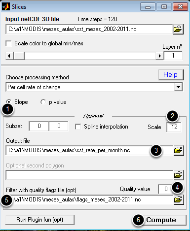
(1) This is the default value and means that we are going to compute the slope of the best fit straight line for each cell across all the 120 months. (2) Because we want the final result in degrees per year and we are using months we need to multiply the final result by 12. (3) is the output file name with the time rate of change. Make sure you provide a meaningful name. If not provided, it will be asked by a separate window. (4) Selects the quality flag to apply to data (For MODIS '0' means retain only the best quality data). (5) Holds the name of the grid with the quality flags. We obtain one such grid by running the "Make a stack of L3 MODIS files" Lesson with a "sds2" parameter to select Qualities instead of SSTs. At the end, hit (5) and provide a file name to save the result.
SST variation in degrees per year
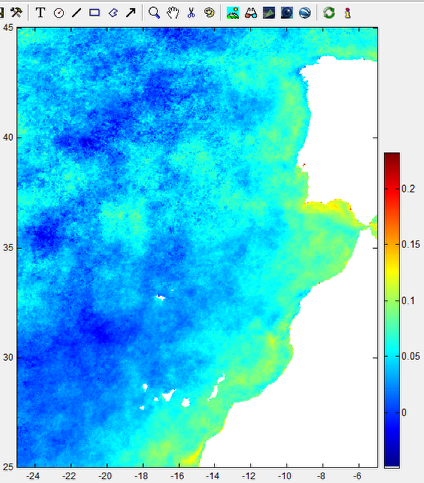
This is what we get.
Compute the time rate on a per-year basis
REPEAT STEP 2 ABOVE BUT MAKE SURE YOU LOADED THE ANNUAL MEANS FILE.
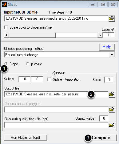
(1) Again, this the default choice. (2) Output file name. Also again, make sure you give a meaningful name. (3) Compute
Note, we don't need to use the "Flags" file because we already used it to compute the annual means composition. We also don't need to apply a scale factor because base data are now the annual means.
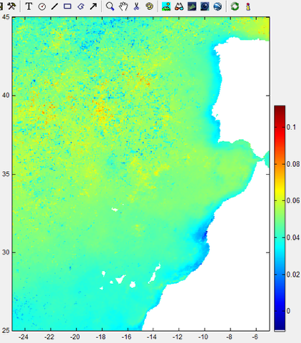
SST variation in degrees per year (second version)
And again, this what we get. Note that it looks quite different from version one but that is because of the automatic color scheme that is based on grid's mea/max. However, they are actually different and to appreciate that, nothing like to compute the difference between the two.
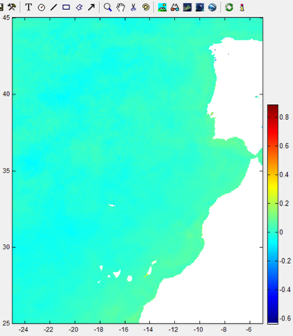
The difference between the two estimates
Why aren't they equal and by consequence their differences be zero (think of it)?
The noisy content on the 'reddish' part makes me think that there was some problem with the quality flags grid and that the correction was not done correctly.