Seismicity from the ISC Bulletin - Part II
Display the vertical distribution of seismicity along the South American - Pacific subduction zone
Load one grid with the South American - Pacific bathymetry/topography
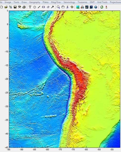
The example used here is a subsample of the etopo2 grid at 4 minutes resolution.
Plot the seismicity of events with magnitude >= 4 for the period 2005/2011
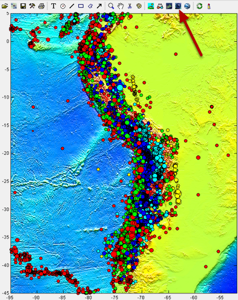
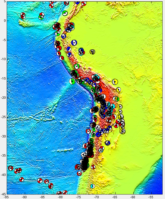
Please refer to the example "Seismicity from the ISC Bulletin - Part I" on how to select/prepare a file with seismicity download from the ISC Bulletin. The example in this figure uses data from the period 2005/2011 for events with magnitude >= 4. Red symbols correspond to events shallower than 33 km and yellow events deeper than 300 km. To see the vertical distribution of the seismicity, hit the icon with eye (see arrow). Note that this uses the free Fledermaus IView3D that needs to be installed.
View the 3D picture
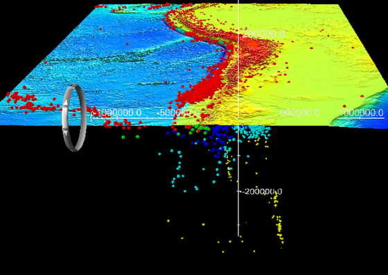
Click-and-drag on the figure to see it from different perspectives
Plot the focal mechanisms
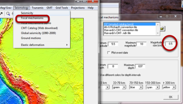
The ISC file also contains the focal mechanisms of the events with magnitude above a certain threshold and we will now plot them. Because this is subduction zone there are lots of focal mechanisms for the 6 years period used in this example. To make such plot, load the the same seismicity file as shown above and change the "Magnitude 5 size (cm)" to 0.5. We also plot only events with magnitude > 5 to no make the figure too heavy.
The focal mechanisms
Looks better when we zoom in
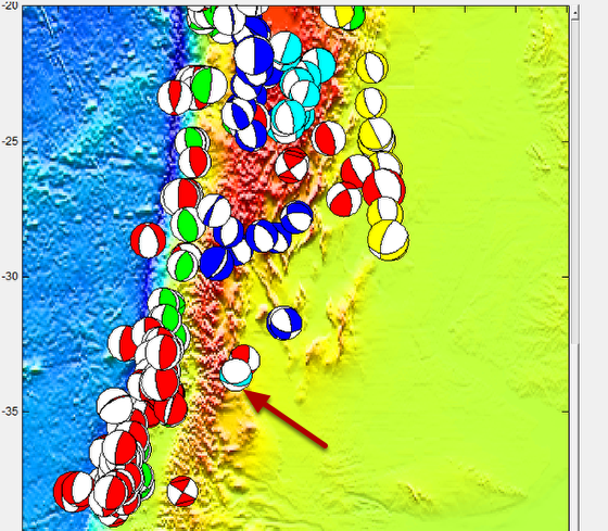
NOTE: You may notice that some mechanisms look wrong like for example the one pointed by the arrow. Well, sorry for that but they are really is Matlab bugs.
Analyze the seismicity along a vertical section
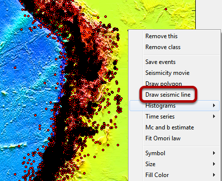
Recreate the seismicity figure but this time do not make the symbols proportional to magnitude. Right-click on any of the red dots to make appear the options shown above. Select the "Draw seismic line" and draw one line like in the next figure.
Set the buffer zone width
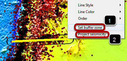
Draw one line like explained on the previous step and right-click on the yellow line to set the buffer zone width. For the example above we used a 0.5 (degrees) buffer zone (1) that will be used to collapse (project) all events inside the buffer on to the yellow line. Finally, right-click on the yellow line again and select "Project seismicity" (2). That creates the next figure.
Cross section
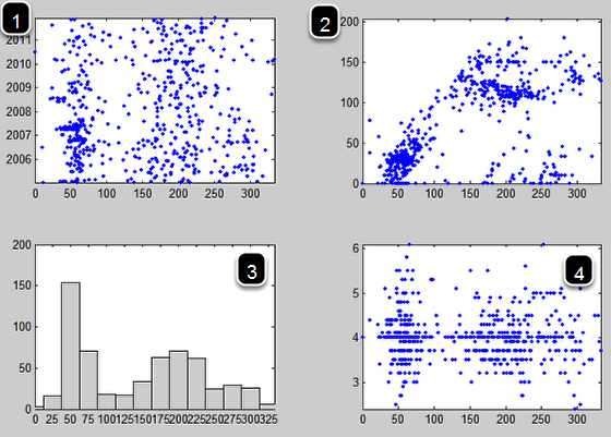
The horizontal axes represents the distance in km along the line. Plot (1) is the distribution of seismicity along time; (2) seismicity in function of depth; (3) is the histogram count on bins with 25 km of width; (4) magnitude of events along the line