Interoperability with (some) other packages
GMT.jl types are plain and not fancy types built around matrices that implement the AbstractArray and Tables interfaces. So, if one wants to make a x,y or x,y,z plot out of data stored in a type with some other internal organization, the simplest is to extract the data in a Mxn matrix and pass it directly to the plot or plot3 or, often even simpler, the viz function.
GMT.jl does not have a recipes system like Plots or Makie but it can still find its way to recognize types that it has no clue what they are. The next three sections show how we can make x,y[,z] plots as well as maps from DataFrames, ODE (SciML) and Rasters types (other commonly used types may be added in future). And that, repeating, without having no clue of what packages implement those types.
DataFrames
As an example, we show an alternative to the Plots solution presented in this SO question
Create and plot a DataFrame
using GMT, DataFrames
df = DataFrame(t = 1:10, series1 = sin.(1:10), series2=rand(10));
plot(df, show=true)
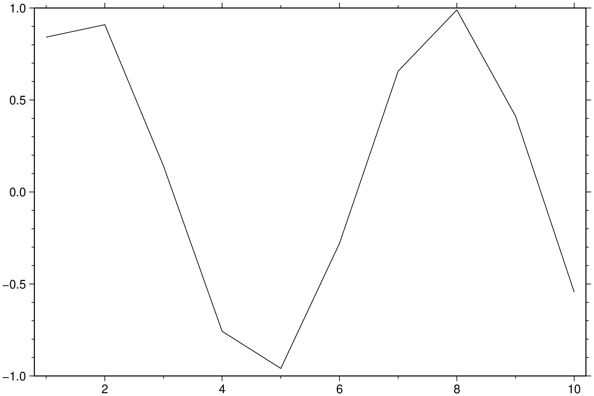
But one problem with the above solution is that although the df has three columns it only plotted a single curve. This happens because in GMT 3rd and on columns may be used to control color, symbol sizes etc and cannot therefore be assumed to plotting data by default. If we want that all columns are interpreted as data, we use the multicol option, like:
using GMT, DataFrames

df = DataFrame(t = 1:10, series1 = sin.(1:10), series2=rand(10));
plot(df, legend=:colnames, multicol=true, show=true)
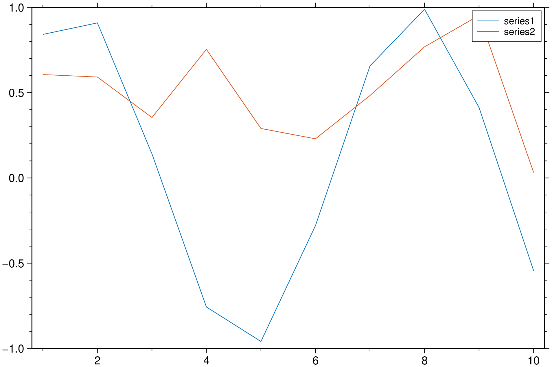
in the example above we took the legend entry from the column names, but if we want to use other labels we can do:
plot(df, legend=("A","B"), multicol=true, show=true)DifferentialEquations
The examples in this section were taken from DifferentialEquations.jl examples
using GMT, DifferentialEquations

function lorenz(du, u, p, t)
	du[1] = p[1] * (u[2] - u[1])
	du[2] = u[1] * (p[2] - u[3]) - u[2]
	du[3] = u[1] * u[2] - p[3] * u[3]
end

u0 = [1.0, 5.0, 10.0];
tspan = (0.0, 100.0);
p = (10.0, 28.0, 8 / 3);
prob = ODEProblem(lorenz, u0, tspan, p);
sol = solve(prob);

plot(sol, multi=true, legend=:colnames, show=true)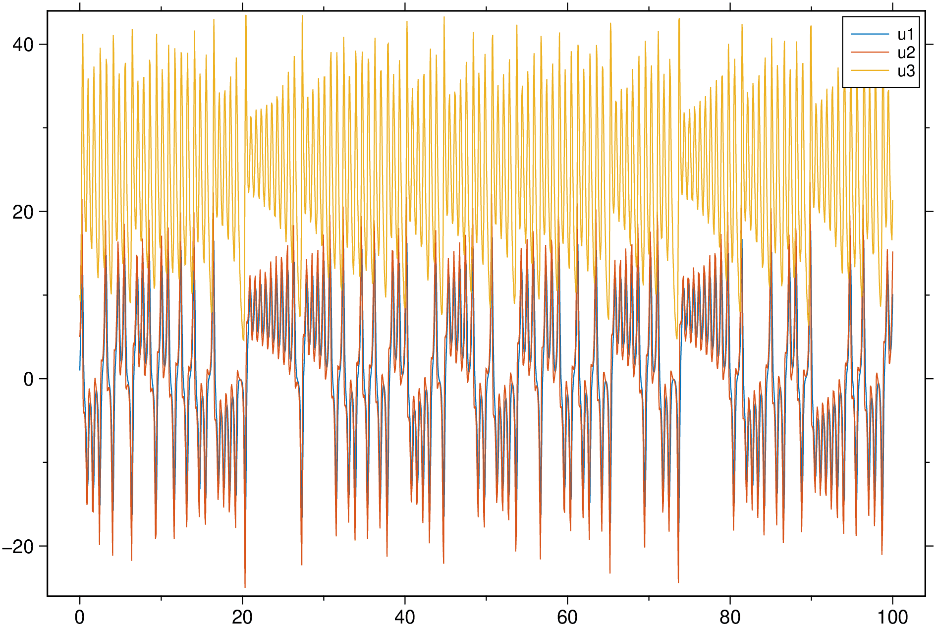
If we make a 3D plot of the sol result, we get the following because first dimension in the converted type is the time.
plot3(sol, show=true)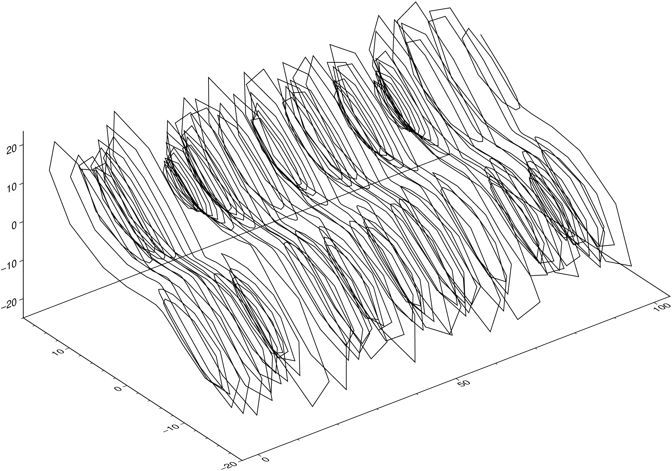
To plot the parametric curve with the three u1, u2, u3 components, we do:
plot3(sol, x=:u1, y=:u2, z=:u3, show=true)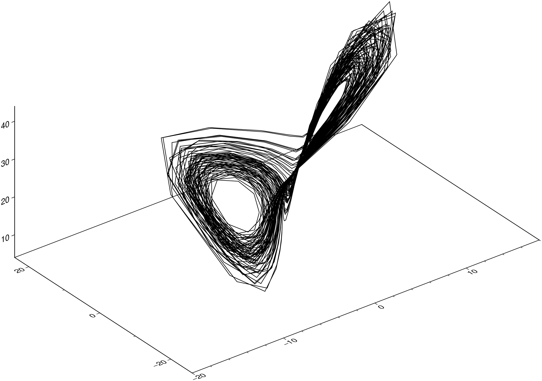
To interpolate the solution (must be done manually) at 5 times more points that original, do:
plot3(sol, x=:u1, y=:u2, z=:u3, interp=5, show=true)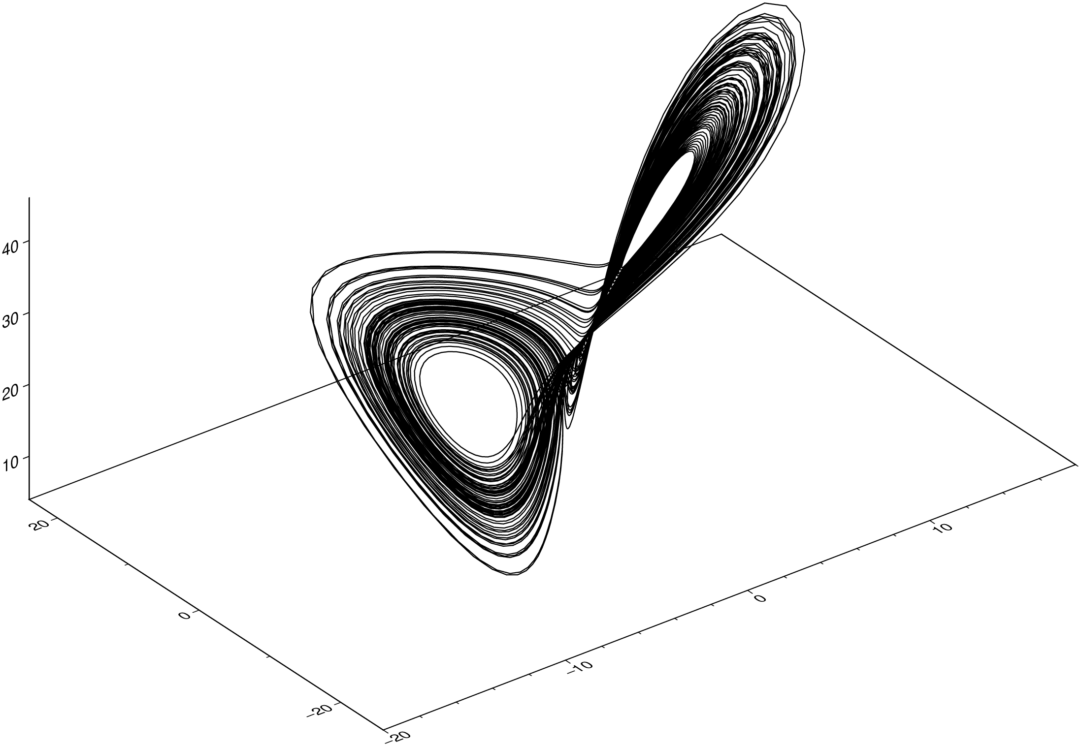
Rasters
Though many of the use cases shown could be reproduced by GMT.jl directly (it also reads netCDF and multi-layred files) the Rasters.jl package is able to keep some metadata (namely the time axis) and lazy reading of large files that GMT is not yet able to match. Here we will reproduce some of the examples from this Rasters.jl docs.
using GMT
using Rasters, RasterDataSources, ArchGDAL

ENV["RASTERDATASOURCES_PATH"] = tempdir();
A = Raster(WorldClim{BioClim}, 5);
viz(A, colorbar=true)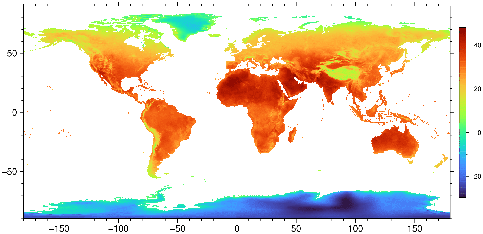
using GMT, Rasters
import NCDatasets

url = "https://archive.unidata.ucar.edu/software/netcdf/examples/tos_O1_2001-2002.nc";
filename = download(url, "tos_O1_2001-2002.nc");
A = Raster(filename);
viz(A[Ti=6], proj=:guess, coast=true, colorbar=true)

viz(A[Ti=1:6], proj=:Robinson, coast=true, colorbar=true)

But I Don't like Kelvins. Fine, want centigrade? Just offset the z values.
G = mat2grid(A[Ti=1:6], offset=-273.15);
viz(G, proj=:Robinson, coast=true, colorbar=true)

These docs were autogenerated using GMT: v1.33.1