band
band(cmd0::String="", arg1=nothing; width=0.0, envelope=false, kwargs...)

or

band(arg1, ag2, arg3; kwargs...)

or

band(Function, range; width=0.0, envelope=false, kwargs...)
Plot a line with a symmetrical or asymmetrical band around it. If the band is not color filled then, by default, only the envelope outline is plotted.
First form expects either a file name or a Matrix/GMTdatset with two to four columns. When number of columns is two, width must be set and can be a scalar (symmetrical band) or a two elements tuple/array with dx & dy offsets (asymmetrical band). A three columns input automatically selects a symmetrical band with offsets taken from third column. A four columns input needs to be disambiguated with the width or envelope options.
Second form expects arg1 to contain a Mx2 array (can be a GMTdataset) with x,y coordinates and upper and lower band limits provided in the arg1 and arg2 vectors (that need to have same number of elements as rows in arg1).
Third form let user pass a function whose x limits are set by the range positional option. When range is a scalar it is interpreted to mean x = linspace(-range, range, 200). A two elements mean x = linspace(-range[1], range[2], 200)
This module is a subset of plot to make it simpler to draw band plots. So not all (fine) controlling parameters are not listed here. For the finest control, user should consult the plot module.
Parameters
B or axes or frame
Set map boundary frame and axes attributes. Default is to draw and annotate left, bottom and vertical axes and just draw left and top axes. More at frame
J or proj or projection : – proj=<parameters>
Select map projection. More at proj
R or region or limits : – limits=(xmin, xmax, ymin, ymax) | limits=(BB=(xmin, xmax, ymin, ymax),) | limits=(LLUR=(xmin, xmax, ymin, ymax),units="unit") | ...more
Specify the region of interest. More at limits. For perspective view view, optionally add zmin,zmax. This option may be used to indicate the range used for the 3-D axes. You may ask for a larger w/e/s/n region to have more room between the image and the axes.
G or fill
Select color or pattern for filling the band [Default is no fill]. Note that plot will search for fill and pen settings in all the segment headers (when passing a GMTdaset or file of a multi-segment dataset) and let any values thus found over-ride the command line settings (but those must be provided in the terse GMT syntax). See Setting color for extend color selection (including color map generation).
L or polygon : – polygon=(sym=true, asym=true, envelope=true, pen=pen)
Add modifiers to build a band polygon from a line segment. Note, this is an alternative way of setting the band that is provided only because it also allows a fine control for the pen band outline.sym=true to build symmetrical envelope around y(x) using deviations dy(x) given in extra column 3.
asym=true to build asymmetrical envelope around y(x) using deviations dy1(x) and dy2(x) from extra columns 3-4.
envelope=true to build asymmetrical envelope around y(x) using bounds yl(x) and yh(x) from extra columns 3-4.
Polygon may be painted (fill) and optionally outlined by adding pen=pen.
envelope : – envelope=true
When input table has four columns, or theband([x y], upper, lower, ...)form is used builds an asymmetrical envelope around y(x) using bounds yl(x) and yh(x) from extra columns 3-4 or the upper & lower vectors are provided as input arguments.
width : – width=val | width=(dx,dy)
Create a symmetrical envelope around y(x) using deviations +/- val or dx & dy. Note: this assumes that the input table has only two columns, otherwise the band type is determined by the number of columns (symmetrical if ncols = 3, asymmetrical if ncols = 4 with type depending on envelope is true or not.)
W or pen=
pen
Set pen attributes for the arrow stem [Defaults: width = default, color = black, style = solid]. See Pen attributes and Vector attributes for arrow line terminations.
U or time_stamp : – time_stamp=true | time_stamp=(just="code", pos=(dx,dy), label="label", com=true)
Draw GMT time stamp logo on plot. More at timestamp
V or verbose : – verbose=true | verbose=level
Select verbosity level. More at verbose
X or xshift or x_offset : xshift=true | xshift=x-shift | xshift=(shift=x-shift, mov="a|c|f|r")
Shift plot origin. More at xshift
Y or yshift or y_offset : yshift=true | yshift=y-shift | yshift=(shift=y-shift, mov="a|c|f|r")
Shift plot origin. More at yshift
figname or savefig or name : – figname=
name.png
Save the figure with thefigname=name.extwhereextchooses the figure image format.
Examples
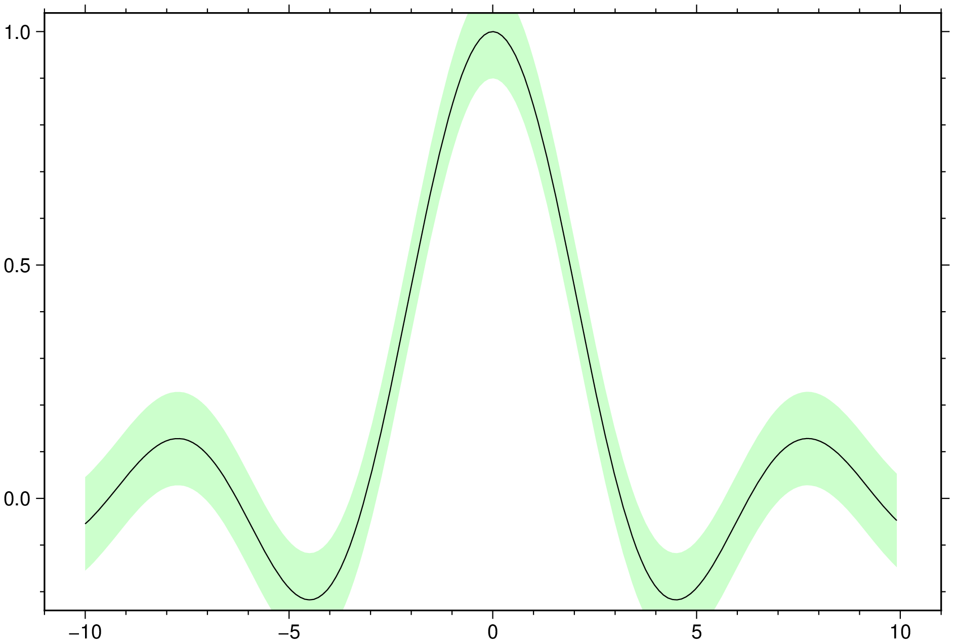
Plot the sinc function with a green band of width 0.1 (above and below the sinc line)
using GMT
x = y = -10:0.11:10;
band(x, sin.(x)./x, width=0.1, fill="green@80", show=true)
These docs were autogenerated using GMT: v1.33.1