clip

clip(cmd0::String="", arg1=[]; kwargs...)

keywords: GMT, Julia, clip paths

Initialize or terminate polygonal clip paths

Description

Reads (x,y) tables (or a file) and draws polygons that are activated as clipping paths. Several files may be read to create complex paths consisting of several non-connecting segments. Only marks that are subsequently drawn inside the clipping path will be shown. To determine what is inside or outside the clipping path, we use the even-odd rule. When a ray drawn from any point, regardless of direction, crosses the clipping path segments an odd number of times, the point is inside the clipping path. If the number is even, the point is outside. The invert option, reverses the sense of what is the inside and outside of the paths by plotting a clipping path along the map boundary. After subsequent plotting, which will be clipped against these paths, the clipping may be deactivated by running the module a second time with the endclip option only.

Required Arguments

• table
  One or more data tables holding a number of data columns.

• C or endclip : – endclip=true or endclip=n
  Mark end of existing clip path(s). No input file will be processed. No projection information is needed unless frame has been selected as well. With no arguments we terminate all active clipping paths. Experts may restrict the termination to just n of the active clipping path by passing that as the argument.

• J or proj or projection : – proj=<parameters>
  Select map projection. More at proj

• R or region or limits : – limits=(xmin, xmax, ymin, ymax) | limits=(BB=(xmin, xmax, ymin, ymax),) | limits=(LLUR=(xmin, xmax, ymin, ymax),units="unit") | ...more
  Specify the region of interest. More at limits. For perspective view view, optionally add zmin,zmax. This option may be used to indicate the range used for the 3-D axes. You may ask for a larger w/e/s/n region to have more room between the image and the axes.

• R or region or limits : – limits=(xmin, xmax, ymin, ymax, zmin, zmax) | limits=(BB=(xmin, xmax, ymin, ymax, zmin, zmax),) | ...more
  Specify the region of interest. Default limits are computed from data extents. More at limits

• A or steps : – steps=true | steps=:meridian|:parallel|:x|:y|:r|:theta
  By default, geographic line segments (as indicated for example by the colinfo option) are drawn as great circle arcs. To draw them as straight lines, use the steps=true. Alternatively, use steps=:meridian to draw the line by first following a meridian, then a parallel. Or append steps=:parallel to start following a parallel, then a meridian. (This can be practical to draw a line along parallels, for example). For Cartesian data, points are simply connected, unless you use steps=:x or steps=:y to draw stair-case curves that whose first move is along x or y, respectively. If your Cartesian data are polar (theta, r), use steps=:t or steps=:r to construct stair-case paths whose first move is along theta or r, respectively.

• B or axes or frame
  Set map boundary frame and axes attributes. Default is to draw and annotate left, bottom and vertical axes and just draw left and top axes. More at frame

• N or invert : – invert=true
  Invert the sense of what is inside and outside. For example, when using a single path, this means that only points outside that path will be shown. Cannot be used together with frame.

• T or clipregion : – clipregion=
  Rather than depending on input data, simply turn on clipping for the current map region. Cannot be used together with frame.

• U or time_stamp : – time_stamp=true | time_stamp=(just="code", pos=(dx,dy), label="label", com=true)
  Draw GMT time stamp logo on plot. More at timestamp

• V or verbose : – verbose=true | verbose=level
  Select verbosity level. More at verbose

• W or pen=pen
  Set pen attributes for the arrow stem [Defaults: width = default, color = black, style = solid]. See Pen attributes

• X or xshift or x_offset : xshift=true | xshift=x-shift | xshift=(shift=x-shift, mov="a|c|f|r")
  Shift plot origin. More at xshift

• Y or yshift or y_offset : yshift=true | yshift=y-shift | yshift=(shift=y-shift, mov="a|c|f|r")
  Shift plot origin. More at yshift

• bi or binary_in : – binary_in=??
  Select native binary format for primary table input. More at

• di or nodata_in : – nodata_in=??
  Substitute specific values with NaN. More at

• e or pattern : – pattern=??
  Only accept ASCII data records that contain the specified pattern. More at

• f or colinfo : – colinfo=??
  Specify the data types of input and/or output columns (time or geographical data). More at

• g or gap : – gap=??
  Examine the spacing between consecutive data points in order to impose breaks in the line. More at

• h or header : – header=??
  Specify that input and/or output file(s) have n header records. More at

• i or incol or incols : – incol=col_num | incol="opts"
  Select input columns and transformations (0 is first column, t is trailing text, append word to read one word only). More at incol

• p or view or perspective : – view=(azim, elev)
  Default is viewpoint from an azimuth of 200 and elevation of 30 degrees.
  Specify the viewpoint in terms of azimuth and elevation. The azimuth is the horizontal rotation about the z-axis as measured in degrees from the positive y-axis. That is, from North. This option is not yet fully expanded. Current alternatives are:

  • view=??
    A full GMT compact string with the full set of options.

  • view=(azim,elev)
    A two elements tuple with azimuth and elevation

  • view=true
    To propagate the viewpoint used in a previous module (makes sense only in bar3!)

  More at perspective

• q or inrows : – inrows=??
  Select specific data rows to be read and/or written. More at

• t or transparency or alpha: – alpha=50
  Set PDF transparency level for an overlay, in (0-100] percent range. [Default is 0, i.e., opaque]. Works only for the PDF and PNG formats.

• yx : – yx=true
  Swap 1st and 2nd column on input and/or output. More at

Examples

To see the effect of a simple clip path which result in some symbols being partly visible or missing altogether, try:

using GMT
clip([0 0; 5 1; 5 5], region=(0,6,0,6), figscale=2.5, pen=(1,:blue))
plot!("@tut_data.txt", fill=:red, marker=:circ, ms=2, region=:same)
clip!(endclip=true, frame=:same, show=true)

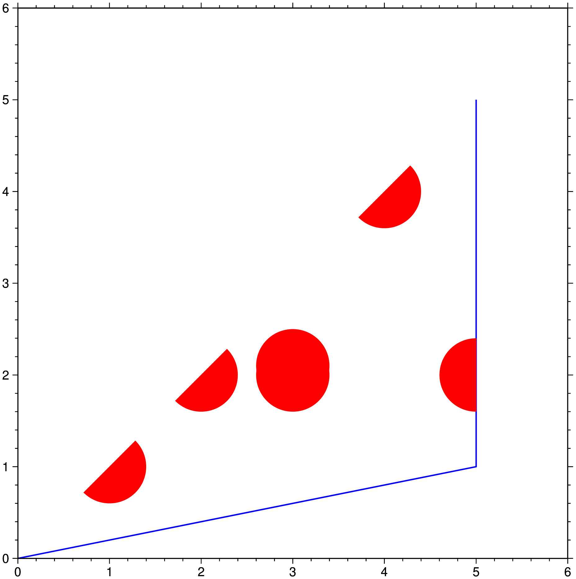
where we activate and deactivate the clip path. Note we also draw the outline of the clip path to make it clear what is being clipped.

See Also