cornerplot
cornerplot(data; kwargs...)Takes a nSamples-by-nDimensions array, and makes density plots of every combination of the dimensions. Plots as a triangular matrix of subplots showing the correlation among input variables. Input data can be a MxN matrix, a GMTdataset or a file name that upon reading with gmtread returns a GMTdataset.
The plot consists of histograms of each column along the diagonal and scatter or hexagonal bining plots for the inter-variable relations, depending on if the the number of samples is <= 1000. But this can be changed with options in kwargs.
cornerplot(data) plots every 2D projection of a multidimensional data set.
cornerplot(..., varnames) prints the names of each dimension. varnames is a vector of strings of length nDimensions. If not provided, column names in the GMTdaset are used.
cornerplot(..., truths) indicates reference values on the plots. Note that truthsmust be a vector of length n dimensions, that is, number of columns in input data.
cornerplot(..., quantile) list of fractional quantiles to show on the 1-D histograms as vertical dashed lines.
marginalhist(..., hexbin=true) Force hexbin plots even when number of points <= 1000. Default hexagon sizes are set via an heuristic rule but can be explicitly set via binstats options, Namely inc or nbins options.
cornerplot(..., scatter=true) Force scatter plots even when number of points > 1000.
cornerplot(..., histcolor|histfill=color) To paint diagonal histograms with a selected color (histcolor=:none to no paint).
cornerplot(...,xvar,yvar) plots the variables xvar and yvar from the table D. You can specify one or multiple variables for yvar and one only for xvar.
Several other options can be used through kwargs to control plot details. Namelly options to fine control the subplots sizes and that are passed to subplot. Options to control the number of bins, and thresholds on countings, passed to binstats. Or options to change markers, marker size and or color, colormap, etc, passed to plot. See examples bellow.
Common options
U or time_stamp : – time_stamp=true | time_stamp=(just="code", pos=(dx,dy), label="label", com=true)
Draw GMT time stamp logo on plot. More at timestamp
V or verbose : – verbose=true | verbose=level
Select verbosity level. More at verbose
X or xshift or x_offset : xshift=true | xshift=x-shift | xshift=(shift=x-shift, mov="a|c|f|r")
Shift plot origin. More at xshift
Y or yshift or y_offset : yshift=true | yshift=y-shift | yshift=(shift=y-shift, mov="a|c|f|r")
Shift plot origin. More at yshift
figname or savefig or name : – figname=
name.png
Save the figure with thefigname=name.extwhereextchooses the figure image format.
Examples
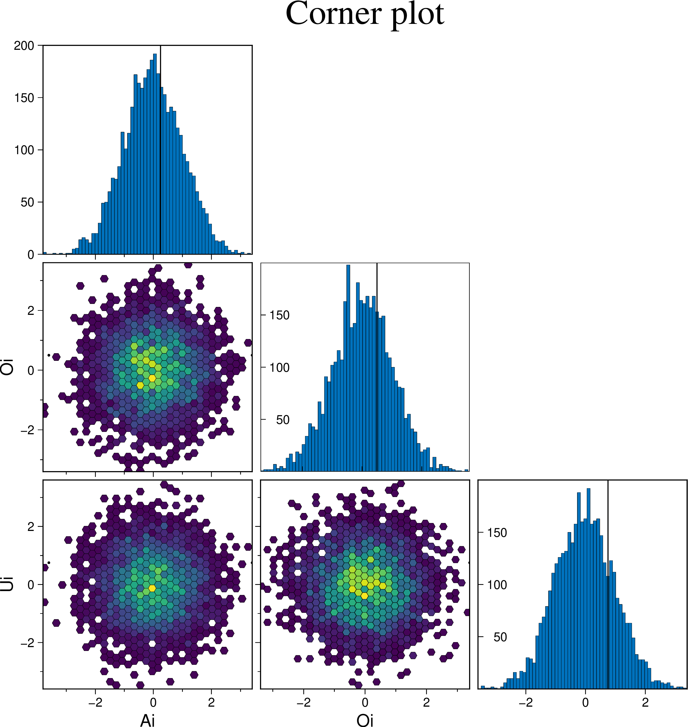
Create a cornerplot plot with hexagonal bins, setting the color map, the vriable names, plot truth and title.
using GMT
cornerplot(randn(4000,3), cmap=:viridis, truths=[0.25, 0.5, 0.75],
           varnames=["Ai", "Oi", "Ui"], title="Corner plot", show=true)
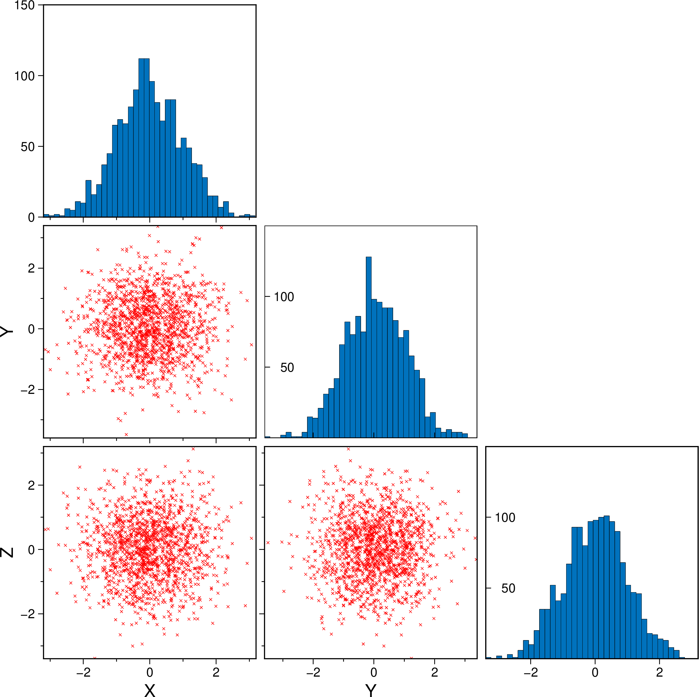
Example on how to control the symbol types, size and color.
using GMT
cornerplot(randn(1500,3), scatter=true, marker=:cross, mec=:red, ms="3p", show=true)
See Also
binstats, histogram, marginalhist, plot
These docs were autogenerated using GMT: v1.33.1