fill_between

fill_between(D1 [,D2]; kwargs...)

keywords: GMT, Julia, area fill plots

Fill the area between two horizontal curves.

The curves are defined by the points (x, y1, y2) in matrix or GMTdataset D1. This creates one or multiple polygons describing the filled area. Alternatively, give a second matrix, D2 (or a scalar y=cte) and the polygons are constructed from the intersections of curves D1 and D2. The D1 arg can also be a file name of a file that can be read with gmtread and return a GMTdataset Note: D1 and D2 do not need to have the same number of points but they should have the same xx limits (or close), otherwise results my look weird.

fill_between(D1) Plots two curves x,y1,y2 and fills the areas bwtween the two curves.

fill_between(..., fill=colors) Give a list with two colors to paint the 'up' and 'down' polygons. Example, fill=(:yellow, :brown)

fill_between(..., fillalpha=[alpha1,alpha2]): Sets the transparency of the two sets of polygons (default 60%). alpha1 and alpha2 are numbers between [0-1] or [0-100], where 1 or 100 mean full transparency.

fill_between(..., pen=...): Sets pen specifications for the two curves. Easiest is to use the shortcuts lt, lc and ls for the line thickness, color and style like it is used in the plot module.

fill_between(..., markers=true) Add marker points at the data locations. These markers will have the same color as the line they sit on.

fill_between(..., stairs=true) Plot stairs curves instead.

fill_between(..., white=true): Draw a thin white border between the curves and the fills.

fill_between(..., labels=...) Pass labels to use in a legend.

• labels=true wil use the column names in D1 and D2.

• labels="Lab1,Lab2" or labels=["Lab1","Lab2"] (this one can be a Tuple too) use the text in Lab1, Lab2.

fill_between(..., legend=...): If used as the above labels it behaves like wise, but its argument can also be a named tuple with legend=(labels="Lab1,Lab2", position=poscode, box=(...)), where poscode is the same as used in text, e.g. TL means TopLeft and box controls the legend box details. See examples at

fill_between(...,xvar,yvar) plots the variables xvar and yvar from the table D1. You can specify one or multiple variables for yvar and one only for xvar.

Common options

• R or region or limits : – limits=(xmin, xmax, ymin, ymax) | limits=(BB=(xmin, xmax, ymin, ymax),) | limits=(LLUR=(xmin, xmax, ymin, ymax),units="unit") | ...more
  Specify the region of interest. More at limits. For perspective view view, optionally add zmin,zmax. This option may be used to indicate the range used for the 3-D axes. You may ask for a larger w/e/s/n region to have more room between the image and the axes.

• U or time_stamp : – time_stamp=true | time_stamp=(just="code", pos=(dx,dy), label="label", com=true)
  Draw GMT time stamp logo on plot. More at timestamp

• V or verbose : – verbose=true | verbose=level
  Select verbosity level. More at verbose

• X or xshift or x_offset : xshift=true | xshift=x-shift | xshift=(shift=x-shift, mov="a|c|f|r")
  Shift plot origin. More at xshift

• Y or yshift or y_offset : yshift=true | yshift=y-shift | yshift=(shift=y-shift, mov="a|c|f|r")
  Shift plot origin. More at yshift

• figname or savefig or name : – figname=name.png
  Save the figure with the figname=name.ext where ext chooses the figure image format.

Examples

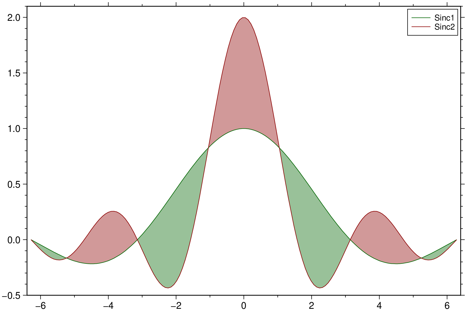
See the intersections of two sinc curves.

using GMT
theta = linspace(-2π, 2π, 150);
y1 = sin.(theta) ./ theta;
y2 = sin.(2*theta) ./ theta;
fill_between([theta y1 y2], legend="Sinc1,Sinc2", show=true)

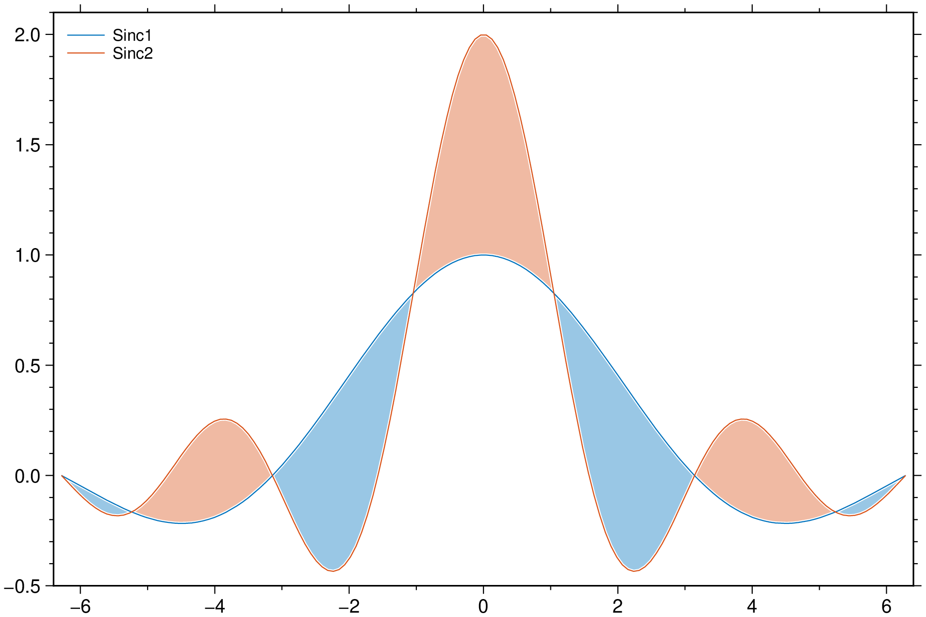
Control the legend position.

using GMT
theta = linspace(-2π, 2π, 150);
y1 = sin.(theta) ./ theta;
y2 = sin.(2*theta) ./ theta;
fill_between([theta y1], [theta y2], fill=("lightblue",:orange), white=true,
             legend=(labels="Sinc1,Sinc2", pos=:TL, box=:none), show=true)

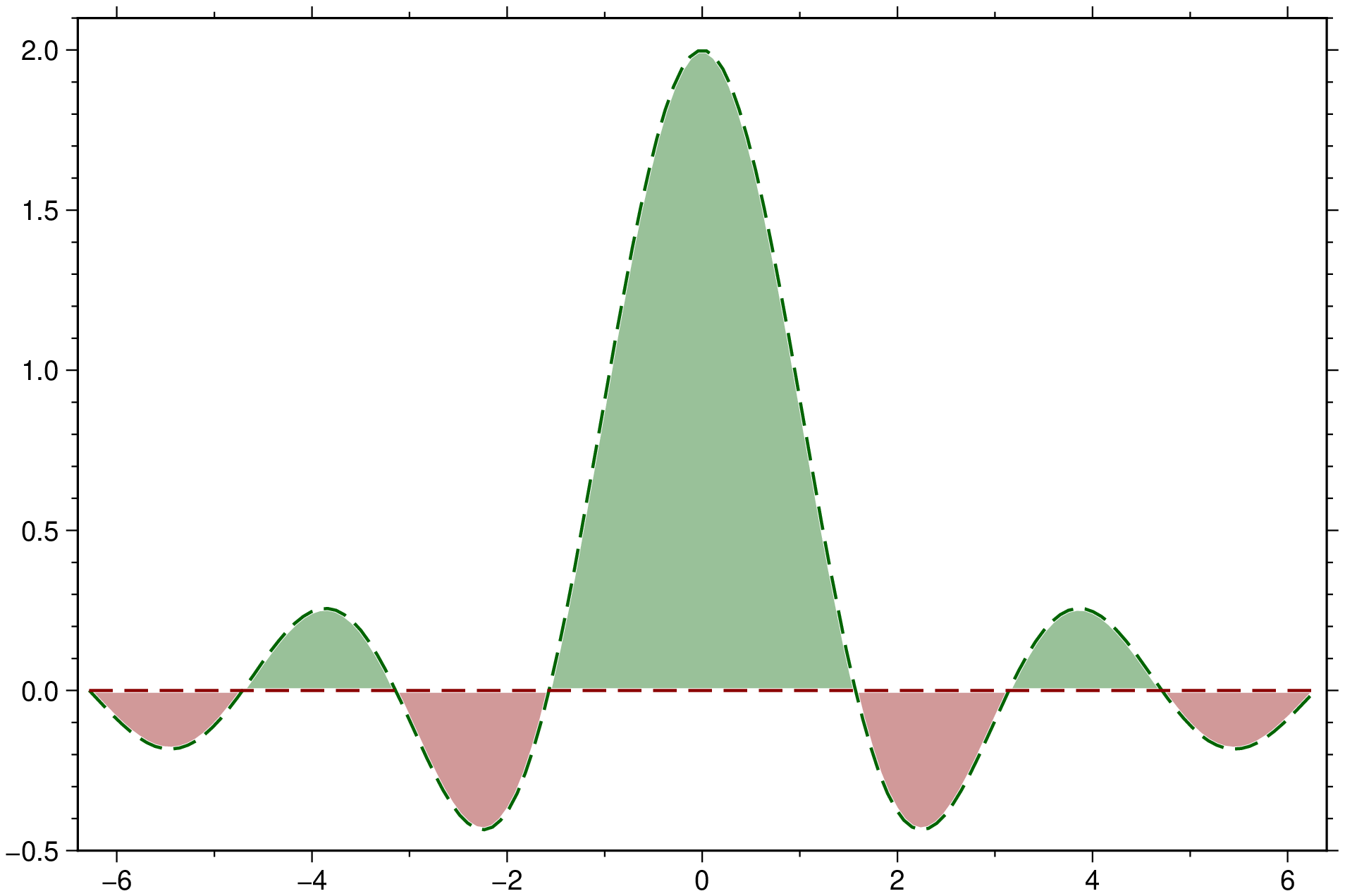
Use a constant y for the second curve.

using GMT
theta = linspace(-2π, 2π, 150);
y2 = sin.(2*theta) ./ theta;
fill_between([theta y2], 0.0, white=true, lt=1, ls=:dash, show=true)

See Also