grdcontour

grdcontour(cmd0::String="", arg1=nothing; kwargs...)

keywords: GMT, Julia, grid contour plots, mapping

Make contour plot or map (using a projection) from a grid.

Read a 2-D grid and produces a contour plot by tracing each contour through the grid. Various options that affect the plotting are available. Alternatively, the x, y, z positions of the contour lines may be saved to one or more output files (or memory) and no plot is produced.

Required Arguments

The 2-D gridded data set to be contoured.

Optional Arguments

• A or annot or annotation : – annot=annot_int | annot=(int=annot_int, disable=true, single=true, labels=labelinfo)
  annot_int is annotation interval in data units; it is ignored if contour levels are given in a file. [Default is no annotations]. Use annot=(disable=true,) to disable all annotations implied by cont. Alternatively do annot=(single=true, int=val) to plot val as a single contour. The optional labelinfo controls the specifics of the label formatting and consists of a named tuple with the following control arguments Label formatting

• B or axes or frame
  Set map boundary frame and axes attributes. Default is to draw and annotate left, bottom and vertical axes and just draw left and top axes. More at frame

• C or cont or contours or levels : – cont=cont_int
  The contours to be drawn may be specified in one of four possible ways:

  1. If cont_int has the suffix ".cpt" and can be opened as a file, it is assumed to be a CPT. The color boundaries are then used as contour levels. If the CPT has annotation flags in the last column then those contours will be annotated. By default all contours are labeled; use annot=(disable=true,)) (or annot=:none) to disable all annotations.

  2. If cont_int is a file but not a CPT, it is expected to contain contour levels in column 1 and a C(ontour) OR A(nnotate) in col 2. The levels marked C (or c) are contoured, while the levels marked A (or a) are contoured and annotated. If the annotation angle is present we will plot the label at that fixed angle [aligned with the contour]. Finally, a contour- specific pen may be present and will override the pen set by pen for this contour level only. Note: Please specify pen in proper format so it can be distinguished from a plain number like angle. If only cont-level columns are present then we set type to C

  3. If cont_int is a constant or an array it means plot those contour intervals. This works also to draw single contours. E.g. contour=[0] will draw only the zero contour. The annot option offers the same list choice so they may be used together to plot a single annotated contour and another single non-annotated contour, as in anot=[10], cont=[5] that plots an annotated 10 contour and an non-annotated 5 contour. If annot is set and cont is not, then the contour interval is set equal to the specified annotation interval.

  4. If no argument is given in modern mode then we select the current CPT.

  5. Otherwise, cont_int is interpreted as a constant contour interval.

If a file is given and ticks is set, then only contours marked with upper case C or A will have tick-marks. In all cases the contour values have the same units as the grid. Finally, if neither cont nor annot are set then we auto-compute suitable contour and annotation intervals from the data range, yielding 10-20 contours.

• D or dump : – dump=fname
  Dump contours as data line segments; no plotting takes place. Append filename template which may contain C-format specifiers. If no filename template is given we write all lines to stdout. If filename has no specifiers then we write all lines to a single file. If a float format (e.g., %6.2f) is found we substitute the contour z-value. If an integer format (e.g., %06d) is found we substitute a running segment count. If an char format (%c) is found we substitute C or O for closed and open contours. The 1-3 specifiers may be combined and appear in any order to produce the the desired number of output files (e.g., just %c gives two files, just %f would separate segments into one file per contour level, and %d would write all segments to individual files; see manual page for more examples.

• -F or force : – force=true | force=:left | force=:right
  Force dumped contours to be oriented so that higher z-values are to the left (force=:left) or right (force=:right) as we move along the contour [Default is arbitrary orientation]. Requires dump.

• G or labels : – labels=()
  The required argument controls the placement of labels along the quoted lines. Choose among five controlling algorithms as explained in Placement methods

• J or proj or projection : – proj=<parameters>
  Select map projection. More at proj

• L or range : – range=(low,high) | range=:n|:p|:N|:P
  Limit range: Do not draw contours for data values below low or above high. Alternatively, limit contours to negative (range=:n) or positive (range=:p) contours. Use upper case N or P to include the zero contour.

• N or fill : – fill=color
  Fill the area between contours using the discrete color table given by color, a Setting color element. Then, cont and annot can be used as well to control the contour lines and annotations. If no color is set (fill=[]) then a discrete color setting must be given via cont instead.

• Q or cut : – cut=np | cut=length&unit[+z]
  Do not draw contours with less than np number of points [Draw all contours]. Alternatively, give instead a minimum contour length in distance units, including c (Cartesian distances using user coordinates) or C for plot length units in current plot units after projecting the coordinates. Optionally, append +z to exclude the zero contour.

• R or region or limits : – limits=(xmin, xmax, ymin, ymax) | limits=(BB=(xmin, xmax, ymin, ymax),) | limits=(LLUR=(xmin, xmax, ymin, ymax),units="unit") | ...more
  Specify the region of interest. More at limits. For perspective view view, optionally add zmin,zmax. This option may be used to indicate the range used for the 3-D axes. You may ask for a larger w/e/s/n region to have more room between the image and the axes.

• S or smooth : – smooth=smoothfactor
  Used to resample the contour lines at roughly every (gridbox_size/smoothfactor) interval.

• T or ticks : – ticks=(local_high=true, local_low=true, gap=gap, closed=true, labels=labels)
  Will draw tick marks pointing in the downward direction every gap along the innermost closed contours only; set closed=true to tick all closed contours. Use gap=(gap,length) and optionally tick mark length (append units as c, i, or p) or use defaults ["15p/3p"]. User may choose to tick only local highs or local lows by specifying local_high=true, local_low=true, respectively. Set labels to annotate the centers of closed innermost contours (i.e., the local lows and highs). If no labels (i.e, set labels="") is set, we use - and + as the labels. Appending exactly two characters, e.g., labels=:LH, will plot the two characters (here, L and H) as labels. For more elaborate labels, separate the low and hight label strings with a comma (e.g., labels="lo,hi"). If a file is given by cont, and ticks is set, then only contours marked with upper case C or A will have tick marks [and annotations]. Note: The labeling of local highs and lows may plot sometimes outside the innermost contour since only the mean value of the ontour coordinates is used to position the label.

• W or pen : – pen=(annot=true, contour=true, pen=pen, colored=true, cline=true, ctext=true)
  annot=true if present, means to annotate contours or contour=true for regular contours [Default]. The pen sets the attributes for the particular line. Default pen for annotated contours: pen=(0.75,:black). Regular contours use pen=(0.25,:black). Normally, all contours are drawn with a fixed color determined by the pen setting. This option may be repeated, for example to separate contour and annotated contours settings. For that the syntax changes to use a Tuple of NamedTuples, e.g. pen=((annot=true, contour=true, pen=pen), (annot=true, contour=true, pen=pen)). If the modifier pen=(cline=true,) is used then the color of the contour lines are taken from the CPT (see cont). If instead pen=(ctext=true,) is appended then the color from the cpt file is applied to the contour annotations. Select pen=(colored=true,) for both effects.

• Z or muladd or scale : – scale=factor | muladd=(factor=factor, shift=shift, periodic=true)
  Use to subtract shift from the data and multiply the results by factor before contouring starts. (Numbers in annot, cont, range refer to values after this scaling has occurred.) Use periodic=true to indicate that this grid file contains z-values that are periodic in 360 degrees (e.g., phase data, angular distributions) and that special precautions must be taken when determining 0-contours.

• U or time_stamp : – time_stamp=true | time_stamp=(just="code", pos=(dx,dy), label="label", com=true)
  Draw GMT time stamp logo on plot. More at timestamp

• V or verbose : – verbose=true | verbose=level
  Select verbosity level. More at verbose

• W or pen=pen
  Set pen attributes for the arrow stem [Defaults: width = default, color = black, style = solid]. See Pen attributes

• X or xshift or x_offset : xshift=true | xshift=x-shift | xshift=(shift=x-shift, mov="a|c|f|r")
  Shift plot origin. More at xshift

• Y or yshift or y_offset : yshift=true | yshift=y-shift | yshift=(shift=y-shift, mov="a|c|f|r")
  Shift plot origin. More at yshift

• figname or savefig or name : – figname=name.png
  Save the figure with the figname=name.ext where ext chooses the figure image format.

Examples

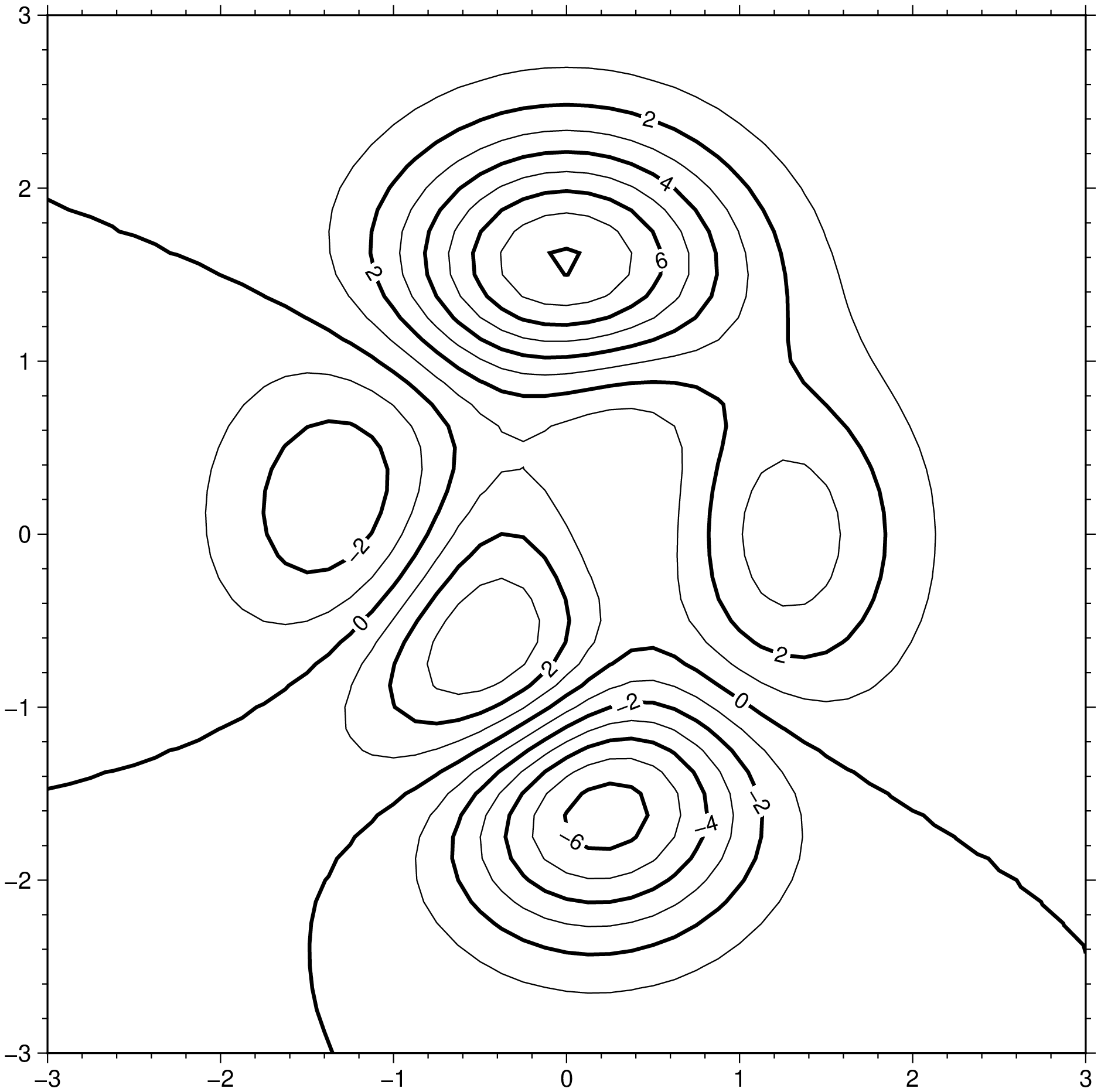
Contour the peaks function. cont=1 and annot=2 means draw contours at every 1 unit of the G grid and annotate at every other contour line:

using GMT
G = GMT.peaks();
grdcontour(G, cont=1, annot=2, show=true)

For a more elaborated example see Contours

See also

The GMT man page