grdcut

grdcut(cmd0::String="", arg1=[], kwargs...)

keywords: GMT, Julia, grid sub-region

Extract subregion from a grid or image

Description

grdcut will produce a new outgrid which is a subregion of ingrid. The subregion may be specified with region as in other programs; the specified range must not exceed the range of ingrid (but see extend). If in doubt, run grdinfo to check range. Alternatively, define the subregion indirectly via a range check on the node values or via distances from a fixed point. Finally, you can use proj for oblique projections to determine the corresponding rectangular region setting that will give a subregion that fully covers the oblique domain. Note: If the input grid is actually an image (gray-scale, RGB, or RGBA), then options extend and z_subregion are unavailable, while for multi-layer Geotiff files only options region, circ_subregion are supported, i.e., you can cut out a sub-region only (which we do via gdal_translate if you have multiple bands). Complementary to grdcut there is grdpaste, which will join together two grid files (not images) along a common edge.

Required Arguments

ingrid : – A grid file name or a Grid type

G or save or outgrid or outfile : – outgrid=[=ID][+ddivisor][+ninvalid][+ooffset|a][+sscale|a][:driver[dataType][+coptions]]
Give the name of the output grid file. Optionally, append =ID for writing a specific file format (See full description). The following modifiers are supported:
- +d - Divide data values by given divisor [Default is 1].
- +n - Replace data values matching invalid with a NaN.
- +o - Offset data values by the given offset, or append a for automatic range offset to preserve precision for integer grids [Default is 0].
- +s - Scale data values by the given scale, or append a for automatic scaling to preserve precision for integer grids [Default is 1].

Note1: Any offset is added before any scaling. +sa also sets +oa (unless overridden). To write specific formats via GDAL, use =gd and supply driver (and optionally dataType) and/or one or more concatenated GDAL -co options using +c. See the “Writing grids and images” cookbook section for more details.

Note2: This is optional and to be used only when saving the result directly on disk. Otherwise, just use the G = modulename(...) form.

R or region or limits : – limits=(xmin, xmax, ymin, ymax) | limits=(BB=(xmin, xmax, ymin, ymax),) | limits=(LLUR=(xmin, xmax, ymin, ymax),units="unit") | ...more
Specify the region of interest. More at limits. For perspective view view, optionally add zmin,zmax. This option may be used to indicate the range used for the 3-D axes. You may ask for a larger w/e/s/n region to have more room between the image and the axes.

Optional Arguments

D or dryrun : – dryrun=true | dryrun="+t"
A "dry run": Simply report the region and increment of what would be the extracted grid given the selected options. No grid is created (|-G| is disallowed) and instead we write a single data record with west east south north xinc yinc to standard output. The increments will reflect the input grid unless it is a remote gridded data set without implied resolution. Append +t to instead receive the information as the trailing string "-Rwest/east/south/north -Ixinc/yinc".

E or rowlice or colslice : – rowlice=coord | colslice=coord
We extract a vertical slice going along the x-column coord or along the y-row coord, depending on the given directive. Note: 1- Input file must be a 3-D netCDF cube, and this option resturns a GMTgrid. 2- coord must exactly match the coordinates given by the cube. We are not interpolating between nodes and only do a clean slice through existing cube nodes. 3- If using the terse GMT syntax (E), then argument must be a string and prefixed with either a x (for extracting a slice along a column) or a y. Example: E="x10.5"

F or clip or cutline : – cutline=polyg | cutline=(polygon=polyg, crop2cutline=true, invert=true)
Specify a multisegment closed polygon file. All grid nodes outside the polygon will be set to NaN. Use the NamedTuple way to say invert=true to invert that and set all nodes inside the polygon to NaN instead. Optionally, add crop2cutline=true to crop the grid region to reflect the bounding box of the polygon.

J or proj or projection : – proj=<parameters>
Select map projection. More at proj

N or extend : – extend=true | extend=nodata
Allow grid to be extended if new region exceeds existing boundaries. Append nodata value to initialize nodes outside current region [Default is NaN].

S or circ_subregion : – circ_subregion=(lon,lat,radius) | circ_subregion="lon/lat/radius+n"
Specify an origin and radius; append a distance unit and we determine the corresponding rectangular region so that all grid nodes on or inside the circle are contained in the subset. If +n is appended (and hence all arg must be a string) we set all nodes outside the circle to NaN.

V or verbose : – verbose=true | verbose=level
Select verbosity level. More at verbose

Z or range : – z_subregion=true | range=(min,max) | range="min/max|+n|N|r"
Determine a new rectangular region so that all nodes outside this region are also outside the given z-range [-inf/+inf]. To indicate no limit on min or max only, specify a hyphen (-) (and hence all arg must be a string). Normally, any NaNs encountered are simply skipped and not considered in the range-decision. Append +n (arg must be a string too) to consider a NaN to be outside the given z-range. This means the new subset will be NaN-free. Alternatively, append +r to consider NaNs to be within the data range. In this case we stop shrinking the boundaries once a NaN is found [Default simply skips NaNs when making the range decision]. Finally, if your core subset grid is surrounded by rows and/or columns that are all NaNs, append +N to strip off such columns before (optionally) considering the range of the core subset for further reduction of the area.

f or colinfo : – colinfo=??
Specify the data types of input and/or output columns (time or geographical data). More at

Units

For map distance unit, append unit d for arc degree, m for arc minute, and s for arc second, or e for meter [Default unless stated otherwise], f for foot, k for km, M for statute mile, n for nautical mile, and u for US survey foot. By default we compute such distances using a spherical approximation with great circles (-jg) using the authalic radius (see PROJ_MEAN_RADIUS). You can use -jf to perform “Flat Earth” calculations (quicker but less accurate) or -je to perform exact geodesic calculations (slower but more accurate; see PROJ_GEODESIC for method used).

Examples

To obtain data for an oblique Mercator projection map we need to extract more data that is actually used. This is necessary because the output of grdcut has edges defined by parallels and meridians, while the oblique map in general does not. Hence, to get all the data from the ETOPO2 data needed to make a contour map for the region defined by its lower left and upper right corners and the desired projection, use:

G = grdcut("@earth_relief_02m", region_diag=(160,20,220,30), proj="oc190/25.5/292/69/1");

Suppose you have used surface to grid ship gravity in the region between 148E - 162E and 8N - 32N, and you do not trust the gridding near the edges, so you want to keep only the area between 150E - 160E and 10N - 30N, then:

G = grdcut("grav_148_162_8_32.nc", region=(150,160,10,30));

To return the subregion of a grid such that any boundary strips where all values are entirely above 0 are excluded, try::

G = grdcut("bathy.nc", z_subregion="-/0");

To return the subregion of a grid such that any boundary rows or columns that are all NaNs, try:

G = grdcut("bathy.nc", z_subregion="+N");

To return the subregion of a grid that contains all nodes within a distance of 500 km from the point 45,30 try:

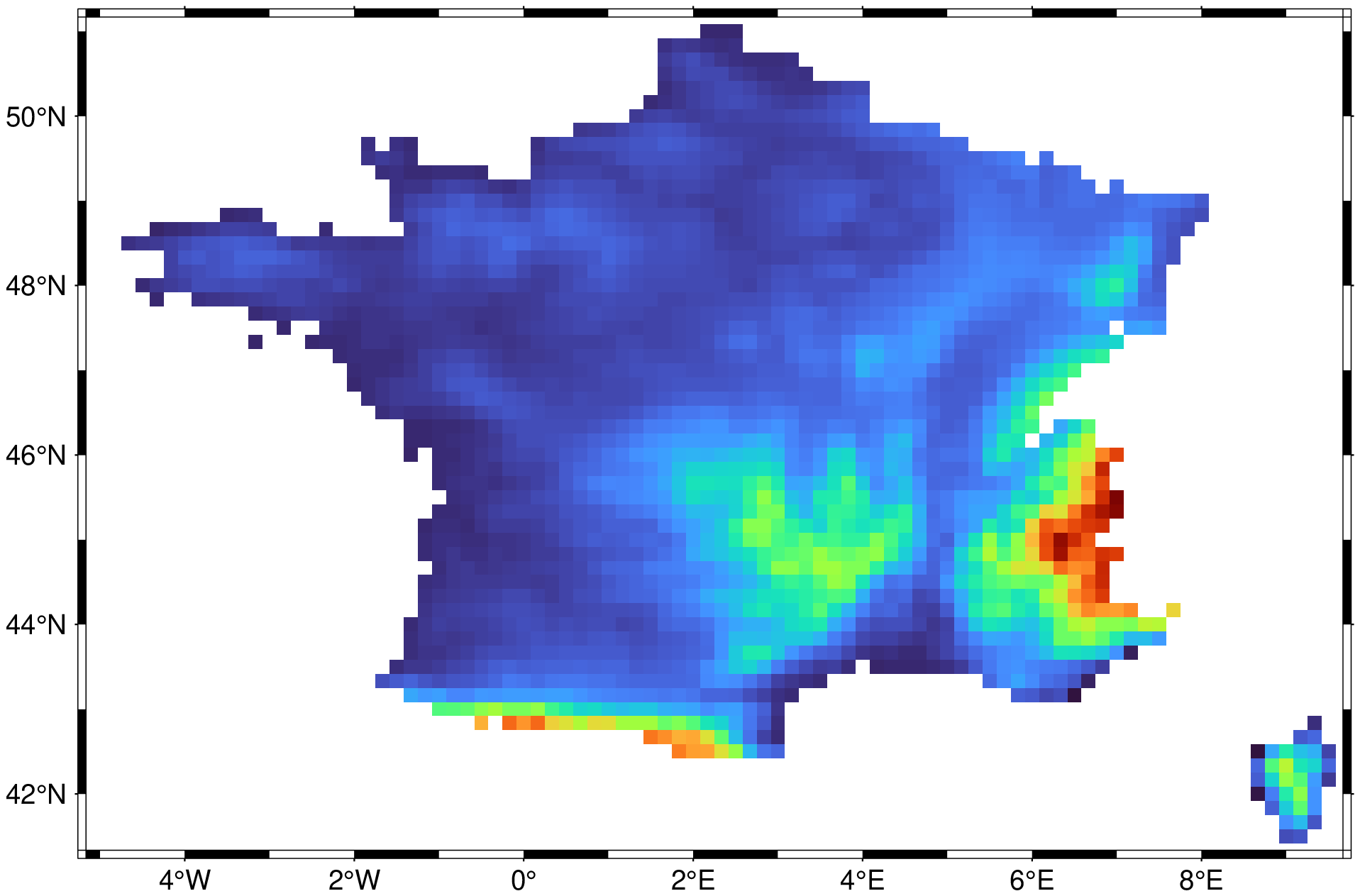
G = grdcutgrdcut("bathy.nc", circ_subregion="45/30/500k");

To create a topography grid with data only inside France and set it to NaN outside France, based on the 10x10 minute DEM, try:

using GMT
D = coast(DCW=:FR, dump=true);
G = grdcut("@earth_relief_10m", cutline=(polygon=D, crop2cutline=true));
imshow(G)

To determine what grid region and resolution (in text format) most suitable for a 24 cm wide map that is using an oblique projection to display the remote Earth Relief data grid, try:

grdcut("@earth_relief", region_diag=(270,20,305,25), proj="Oc280/25.5/22/69/24c", dryrun="+t")

Notes

If the input file is a geotiff with multiple data bands then the output format will depend on your selection (if any) of the bands to keep: If you do not specify any bands (which means we consider all the available bands) or you select more than one band, then the output file can either be another geotiff (if you give a .tif[f] extension) or it can be a multiband netCDF file (if you give a .nc or .grd extension). If you select a single band from the input geotiff then GMT will normally read that in as a single grid layer and thus write a netCDF grid (unless you append another grid format specifier). However, if your output filename has a .tif[f] extension then we will instead write it as a one-band geotiff. All geotiff output operations are done via GDAL's gdal_translate.