grdimage

grdimage(cmd0::String=""; kwargs...)

keywords: GMT, Julia, grid visualization, Geotiff, mapping

Project grids or images and plot them on maps

Description

Reads one 2-D grid and produces a gray-shaded (or colored) map by plotting rectangles centered on each grid node and assigning them a gray-shade (or color) based on the z-value. Alternatively, grdimage reads three 2-D grid files with the red, green, and blue components directly (all must be in the 0-255 range). Optionally, illumination may be added by providing a file with intensities in the (-1,+1) range or instructions to derive intensities from the input data grid. Values outside this range will be clipped. Such intensity files can be created from the grid using grdgradient and, optionally, modified by grdhisteq. A third alternative is available when GMT is build with GDAL support. Pass img which can be an image file (geo-referenced or not). In this case the images can optionally be illuminated with the file provided via the shade option. Here, if image has no coordinates then those of the intensity file will be used.

When using map projections, the grid is first resampled on a new rectangular grid with the same dimensions. Higher resolution images can be obtained by using the -E option. To obtain the resampled value (and hence shade or color) of each map pixel, its location is inversely projected back onto the input grid after which a value is interpolated between the surrounding input grid values. By default bi-cubic interpolation is used. Aliasing is avoided by also forward projecting the input grid nodes. If two or more nodes are projected onto the same pixel, their average will dominate in the calculation of the pixel value. Interpolation and aliasing is controlled with the -n option.

The region option can be used to select a map region larger or smaller than that implied by the extent of the grid.

Required Arguments

• J or proj or projection : – proj=<parameters>
  Select map projection. More at proj

Optional Arguments

• A or img_out or image_out : – img_out=fname
  Save an image in a raster format instead of PostScript. Use extension .ppm for a Portable Pixel Map format. For GDAL-aware versions there are more choices: Use fname to select the image file name and extension. If the extension is one of .bmp, .gif, .jpg, .png, or .tif then no driver information is required. For other output formats you must append the required GDAL driver. The driver is the driver code name used by GDAL; see your GDAL installation's documentation for available drivers. Append a +c<options> string where options is a list of one or more concatenated number of GDAL -co options. For example, to write a GeoPDF with the TerraGo format use "=PDF+cGEO_ENCODING=OGC_BP". Notes: (1) If a tiff file (.tif) is selected then we will write a GeoTiff image if the GMT projection syntax translates into a PROJ4 syntax, otherwise a plain tiff file is produced. (2) Any vector elements will be lost.

• B or axes or frame
  Set map boundary frame and axes attributes. Default is to draw and annotate left, bottom and vertical axes and just draw left and top axes. More at frame

• C or color or cmap or colorap or colorscale : – color=cpt
  Where cpt is a GMTcpt type or a cpt file name (for grd_z only). Alternatively, supply the name of a GMT color master dynamic CPT [turbo] to automatically determine a continuous CPT from the grid's z-range; you may round up/down the z-range by adding +i zinc. Yet another option is to specify color="color1,color2 [,color3 ,...]" or color=((r1,g1,b1),(r2,g2,b2),...) to build a linear continuous CPT from those colors automatically. In this case color1 etc can be a (r,g,b) triplet, a color name, or an HTML hexadecimal color (e.g. #aabbcc ) (see Setting color). When not explicitly set, but a color map is needed, we will either use the current color map, if available (set by a previous call to makecpt), or the default turbo color map.

• clim : – clim=(zmin,zmax) | clim=:zscale
  When doing an automatic colorization (i.e., when a colormap is not provided explicitly), limit the automatic color map to be computed between zmin,zmax. Grid values below z_min and above z_max will be painted with the same color as those. Alternatively, use clim=:zscale to use the Interval based on IRAF’s zscale that is an algorithm used in astronomy for finding colorbar limits of for the grid, which showcase data near the median.

• clip : – clip="land" | clip=:ocean | clip="country_code(s)" | clip=(country="code(s)", [outside=true]) | clip=xy | clip=(xy, inverse=true)
  Clip the image according to the selected option. First set of options do the clipping using the coast module. e.,g.: clip="land" (or =:land) clip outside land areas. clip="ocean" does the inverse. clip="country_code(s)" uses one or more country codes (separated by commas) to do the clipping. If want to reverse the sense of the clipping, use the form clip=(country="code(s)", outside=true). Use clip=(continent=code, [outside=true]) to pass the name of continent. Pay attention that this option must be a named tuple. The second set of options make use of the clip module and expect a first argument with a Mx2 matrix with the coordinates of the clipping polygon.

• coast : – coast=true | coast=(...)
  Call the coast module to overlay coastlines and/or countries. The short form coast=true just plots the coastlines with a black, 0.5p thickness line. To access all options available in the coast module passe them in the named tuple (...).

• colorbar : – colorbar=true | colorbar=(...)
  Call the colorbar module to add a colorbar. The short form colorbar=true automatically adds a color bar on the right side of the image using the current color map stored in the global scope. To access all options available in the colorbar module passe them in the named tuple (...).

• equalize : – equalize=true | equalize=ncolors
  With automatic colorization, map data values to colors through the data’s cumulative distribution function (CDF), so that the colors are histogram equalized. Default (with equalize=true) chooses arbitrary values by a crazy scheme based on equidistant values for a Gaussian CDF. Use equalize=ncolors to specify the desire number of colors.

• percent : – percent=pct
  Exclude the two tails of the distribution (in percentage). Grid values are sorted and we exclude data in 0.5pct and 100 - 0.5pct from the automatic colormap determination. This option is specially useful when the grid has outliers.

• D or img_in or image_in : – img_in=true | img_in=:r
  GMT will automatically detect standard image files (Geotiff, TIFF, JPG, PNG, GIF, etc.) and will read those via GDAL. For very obscure image formats you may need to explicitly set img_in, which specifies that the grid is in fact an image file to be read via GDAL. Use img_in=:r to assign the region specified by region to the image. For example, if you have used region=global then the image will be assigned a global domain. This mode allows you to project a raw image (an image without referencing coordinates).

• E or dpi : – dpi=xx | dpi=:i
  Sets the resolution of the projected grid that will be created if a map projection other than Linear or Mercator was selected [100]. By default, the projected grid will be of the same size (rows and columns) as the input file. Specify dpi=:i to use the PostScript image operator to interpolate the image at the device resolution.

• G : – G="+b" | G="+f"
  This option only applies when a resulting 1-bit image otherwise would consist of only two colors: black (0) and white (255). If so, this option will instead use the image as a transparent mask and paint the mask with the given color. Use G="+b" to paint the background pixels (1) or G="+f" for the foreground pixels [Default].

• I or shade or shading or intensity : – shade=grid | shade=azim | shade=(azimuth=az, norm=params, auto=true)
  Gives the name of a grid with intensities in the (-1,+1) range, or a constant intensity to apply everywhere (affects the ambient light). Alternatively, derive an intensity grid from the input data grid grd_z via a call to grdgradient; use shade=az or shade=(azimuth=az, norm=params) to specify azimuth and intensity arguments for that module or just give shade=true to select the default arguments (azim=-45,norm=:t1). If you want a more specific intensity scenario then run grdgradient separately first.

• M or monochrome : – monochrome=true
  Force conversion to monochrome image using the (television) YIQ transformation. Cannot be used with nan_alpha.

• N or noclip : – noclip=true
  Do not clip the image at the map boundary (only relevant for non-rectangular maps).

• Q or nan_alpha or alpha_color : – nan_alpha=true or alpha_color=true|(r,g,b)
  Make grid nodes with z = NaN transparent. If input is an image alpha_color picks one color (default is black) and makes it transparent (requires GMT6.2 and above).

• R or region or limits : – limits=(xmin, xmax, ymin, ymax) | limits=(BB=(xmin, xmax, ymin, ymax),) | limits=(LLUR=(xmin, xmax, ymin, ymax),units="unit") | ...more
  Specify the region of interest. More at limits. For perspective view view, optionally add zmin,zmax. This option may be used to indicate the range used for the 3-D axes. You may ask for a larger w/e/s/n region to have more room between the image and the axes.

• U or time_stamp : – time_stamp=true | time_stamp=(just="code", pos=(dx,dy), label="label", com=true)
  Draw GMT time stamp logo on plot. More at timestamp

• V or verbose : – verbose=true | verbose=level
  Select verbosity level. More at verbose

• X or xshift or x_offset : xshift=true | xshift=x-shift | xshift=(shift=x-shift, mov="a|c|f|r")
  Shift plot origin. More at xshift

• Y or yshift or y_offset : yshift=true | yshift=y-shift | yshift=(shift=y-shift, mov="a|c|f|r")
  Shift plot origin. More at yshift

• n or interp or interpol : – interp=params
  Select interpolation mode for grids. More at interp

• p or view or perspective : – view=(azim, elev)
  Default is viewpoint from an azimuth of 200 and elevation of 30 degrees.
  Specify the viewpoint in terms of azimuth and elevation. The azimuth is the horizontal rotation about the z-axis as measured in degrees from the positive y-axis. That is, from North. This option is not yet fully expanded. Current alternatives are:

  • view=??
    A full GMT compact string with the full set of options.

  • view=(azim,elev)
    A two elements tuple with azimuth and elevation

  • view=true
    To propagate the viewpoint used in a previous module (makes sense only in bar3!)

  More at perspective

• t or transparency or alpha: – alpha=50
  Set PDF transparency level for an overlay, in (0-100] percent range. [Default is 0, i.e., opaque]. Works only for the PDF and PNG formats.

• figname or savefig or name : – figname=name.png
  Save the figure with the figname=name.ext where ext chooses the figure image format.

Examples

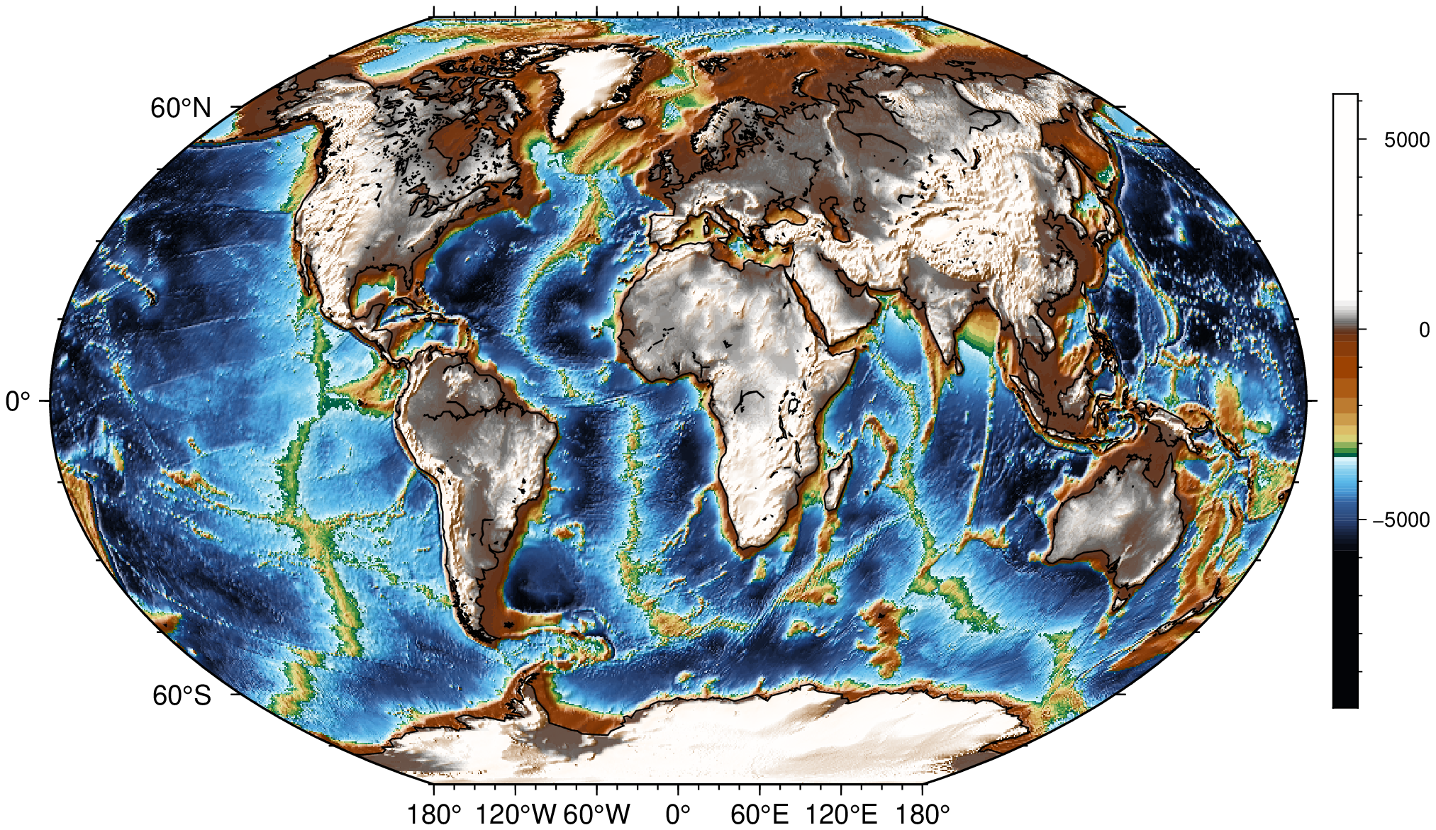
To make a map of a shaded global bathymetry (automatically download it if needed) using the Winkel projection, add coast lines, a colorbar and do an histogram equalization with 64 colors, do:

using GMT
grdimage("@earth_relief_20m_g", proj=:Winkel, equalize=64, coast=true,
         colorbar=true, shade=true, show=true)

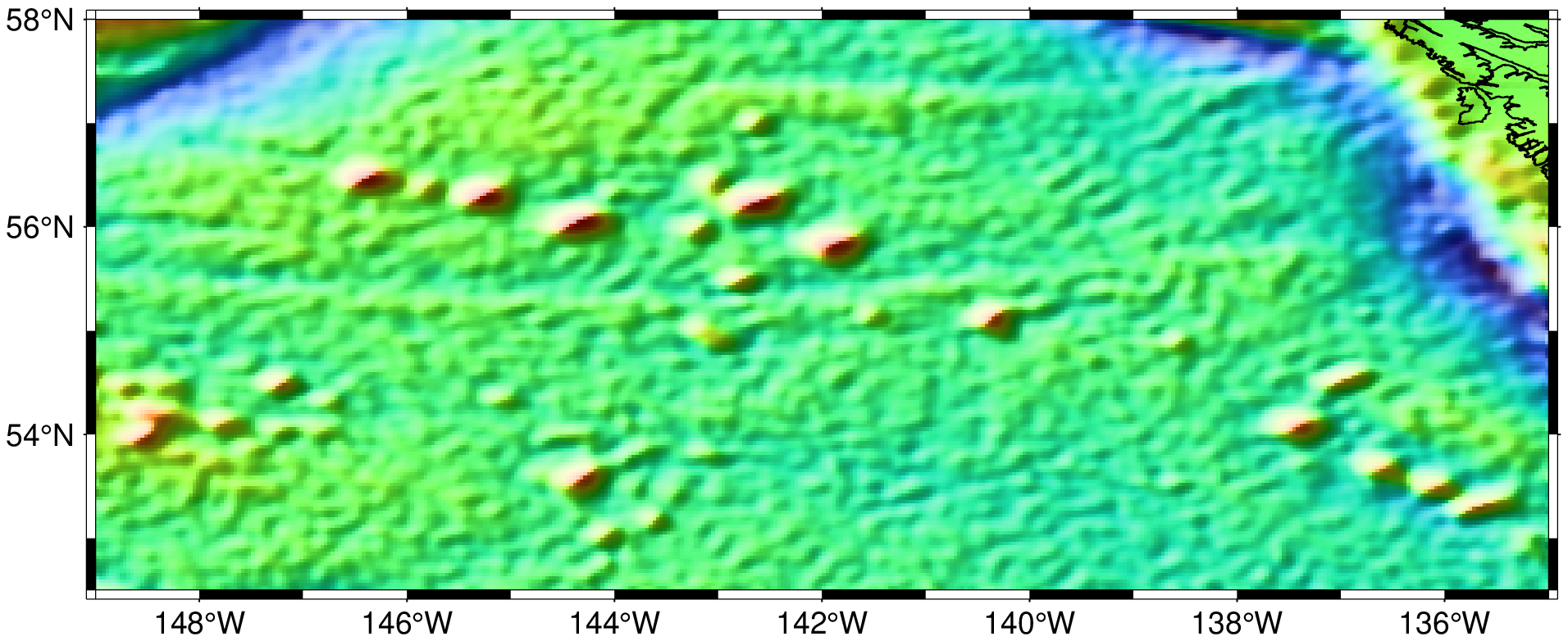
For a quick-and-dirty illuminated color map of the data in the remote file @AKgulfgrav.nc, try:

using GMT
grdimage("@AK_gulf_grav.nc", shade=true, coast=true, show=true)

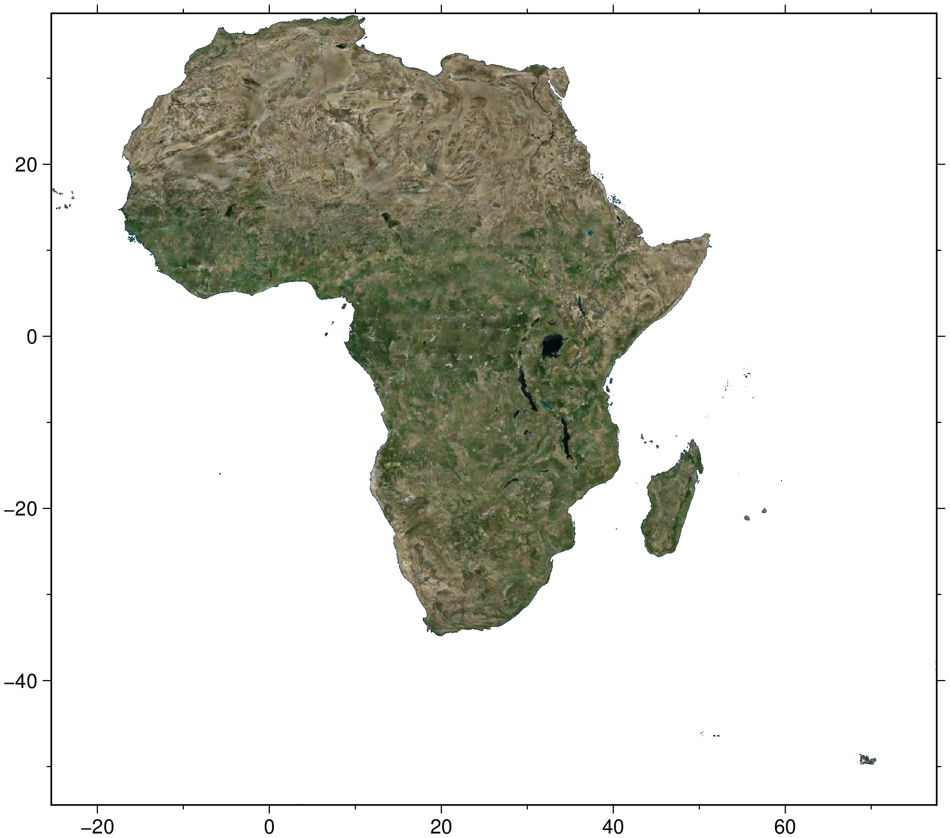
Clip the outside of Africa from Bing mosaic. (You can try also viz(I, clip=:land) and viz(I, clip=(continent=:AF, outside=true)))

using GMT
I = mosaic(region=(continent="AF",));   # Get a mosaic of the ~Africa region
viz(I, clip=(continent=:AF,))           # Clip outside of the African continent.