nearneighbor
nearneighbor(cmd0::String="", arg1=nothing; kwargs...)Grid table data using a "Nearest neighbor" algorithm
Description
Reads randomly-spaced (x,y,z[,w]) triples [quadruplets] from file or table and uses a nearest neighbor algorithm to assign a weighted average value to each node that has one or more data points within a search radius (R) centered on the node with adequate coverage across a subset of the chosen sectors. The node value is computed as a weighted mean of the nearest point from each sector inside the search radius. The weighting function and the averaging used is given by
\[ w(r_i) = \frac{w_i}{1 + d(r_i) ^ 2}, \quad d(r) = \frac {3r}{R}, \quad \bar{z} = \frac{\sum_i^n w(r_i) z_i}{\sum_i^n w(r_i)} \]where n is the number of data points that satisfy the selection criteria and \(r_i\) is the distance from the node to the i'th data point. If no data weights are supplied then \(w_i = 1\).
using GMT

plot([0.75 1.25], region=(0,2,0,2), figscale=4, marker=:circ, ms=5, pen=:thick, fill="lightgreen@70", frame=(grid=0.25,))
d = [0.04 1.8; 0.3 0.3; 0.31 0.7; 0.65 1.88; 0.9 0.44; 0.88 0.2; 1.3 0.8; 1.72 1.1; 1.33 1.59; 1.8 1.9; 1.82 0.5; 1.6 1.3;
# inside but not close enough
0.5	0.9; 0.3 1.3; 0.8 1.7; 0.6 1.65]
plot!(d, marker=:circ, ms=0.25, fill=:black)
plot!([0.52 1.52; 0.6 1.2; 1.15 1.3; 1 0.88], marker=:circ, ms=0.25, fill=:red)
d = [0.75 1.25; 0.5 0.9; NaN NaN; 0.75 1.25; 0.52 1.52; NaN NaN; 0.75 1.25; 0.6 1.2; NaN NaN; 0.75 1.25; 1.15 1.3; NaN NaN; 0.75 1.25; 1 0.88]
plot!(d, pen=:thinnest)
plot!([0.25 1.25; 1.25 1.25; NaN NaN; 0.75 0.75; 0.75 1.75], pen=:thicker)
plot!([0.75 1.25; 1.10355 1.60355], pen=(1,:dash))
text!(mat2ds([1 1.4; 1.03 0.93],["R", "r@-i@-"]), font=(16,"Times-Italic"), justify=:BL)
showfig()
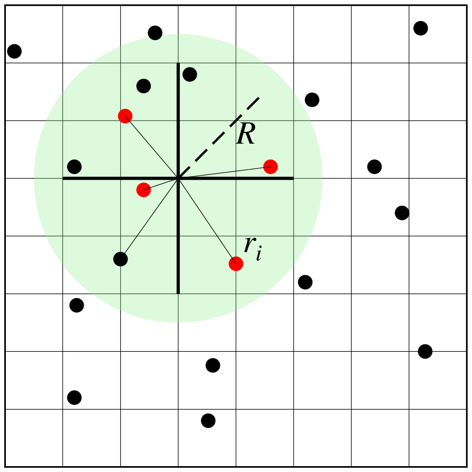
Search geometry includes the search radius (R) which limits the points considered and the number of sectors (here 4), which restricts how points inside the search radius contribute to the value at the node. Only the closest point in each sector (red circles) contribute to the weighted estimate.
Required Arguments
table 3 [or 4, see weights] column data from file or GMTdataset holding (x,y,z[,w]) data values. If no file is specified, nearneighbor will read from standard input.
G or save or outgrid or outfile : – outgrid=[=ID][+ddivisor][+ninvalid][+ooffset|a][+sscale|a][:driver[dataType][+coptions]]
Give the name of the output grid file. Optionally, append=IDfor writing a specific file format (See full description). The following modifiers are supported:+d - Divide data values by given divisor [Default is 1].
+n - Replace data values matching invalid with a NaN.
+o - Offset data values by the given offset, or append a for automatic range offset to preserve precision for integer grids [Default is 0].
+s - Scale data values by the given scale, or append a for automatic scaling to preserve precision for integer grids [Default is 1].
Note1: Any offset is added before any scaling. +sa also sets +oa (unless overridden). To write specific formats via GDAL, use =gd and supply driver (and optionally dataType) and/or one or more concatenated GDAL -co options using +c. See the “Writing grids and images” cookbook section for more details.
Note2: This is optional and to be used only when saving the result directly on disk. Otherwise, just use the G = modulename(...) form.
I or inc or increment or spacing : – inc=x_inc | inc=(xinc, yinc) | inc="xinc[+e|n][/yinc[+e|n]]"
Specify the grid increments or the block sizes. More at spacing
J or proj or projection : – proj=<parameters>
Select map projection. More at proj
R or region or limits : – limits=(xmin, xmax, ymin, ymax) | limits=(BB=(xmin, xmax, ymin, ymax),) | limits=(LLUR=(xmin, xmax, ymin, ymax),units="unit") | ...more
Specify the region of interest. More at limits. For perspective view view, optionally add zmin,zmax. This option may be used to indicate the range used for the 3-D axes. You may ask for a larger w/e/s/n region to have more room between the image and the axes.
S or search_radius : – search_radius=rad
Sets the search_radius that determines which data points are considered close to a node. Append the distance unit (see Units).
Optional Arguments
E or empty : – empty=??
Set the value assigned to empty nodes [NaN].
V or verbose : – verbose=true | verbose=level
Select verbosity level. More at verbose
N or sectors or nn or nearest : – sectors=n_sectors | sectors=(n=n_sectors, min_sectors=n_min)
The circular search area centered on each node is divided into n_sectors sectors. Average values will only be computed if there is at least one value inside each of at least n_min of the sectors for a given node. Nodes that fail this test are assigned the value NaN (but see empty). If min_sectors is omitted then n_min is set to be at least 50% of n_sectors (i.e., rounded up to next integer) [Default is a quadrant search with 100% coverage, i.e., n_sectors = n_min = 4]. Note that only the nearest value per sector enters into the averaging; the more distant points are ignored. Alternatively, use sectors:nn or sectors=:nearest to call GDALʻs nearest neighbor algorithm instead.
W or weights : – weights=true
Input data have a 4th column containing observation point weights. These are multiplied with the geometrical weight factor to determine the actual weights used in the calculations.
a or aspatial : – aspatial=??
Control how aspatial data are handled in GMT during input and output. More at
bi or binary_in : – binary_in=??
Select native binary format for primary table input. More at
di or nodata_in : – nodata_in=??
Substitute specific values with NaN. More at
e or pattern : – pattern=??
Only accept ASCII data records that contain the specified pattern. More at
f or colinfo : – colinfo=??
Specify the data types of input and/or output columns (time or geographical data). More at
g or gap : – gap=??
Examine the spacing between consecutive data points in order to impose breaks in the line. More at
h or header : – header=??
Specify that input and/or output file(s) have n header records. More at
i or incol or incols : – incol=col_num | incol="opts"
Select input columns and transformations (0 is first column, t is trailing text, append word to read one word only). More at incol
n or interp or interpol : – interp=params
Select interpolation mode for grids. More at interp
q or inrows : – inrows=??
Select specific data rows to be read and/or written. More at
r or reg or registration : – reg=:p | reg=:g
Select gridline or pixel node registration. Used only when output is a grid. More at
w or wrap or cyclic : – wrap=??
Convert input records to a cyclical coordinate. More at
yx : – yx=true
Swap 1st and 2nd column on input and/or output. More at
For map distance unit, append unit d for arc degree, m for arc minute, and s for arc second, or e for meter [Default unless stated otherwise], f for foot, k for km, M for statute mile, n for nautical mile, and u for US survey foot. By default we compute such distances using a spherical approximation with great circles (-jg) using the authalic radius (see PROJ_MEAN_RADIUS). You can use -jf to perform “Flat Earth” calculations (quicker but less accurate) or -je to perform exact geodesic calculations (slower but more accurate; see PROJ_GEODESIC for method used).
Examples
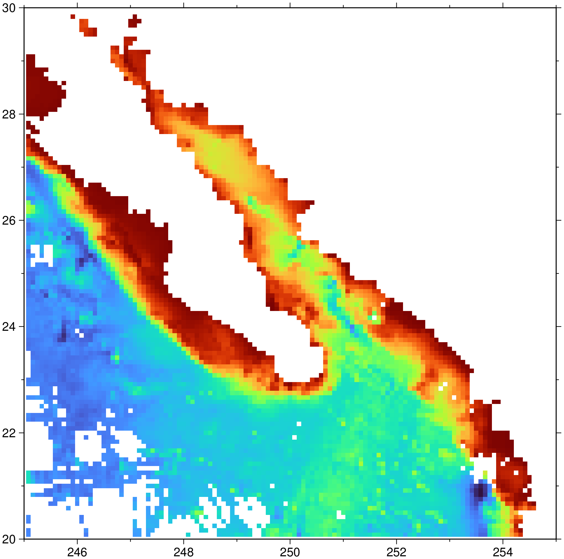
To grid the data in the remote file @ship_15.txt at 5x5 arc minutes using a search radius of 15 arch minutes, and plot the resulting grid using default projection and colors, do
using GMT
G = nearneighbor("@ship_15.txt", region=(245,255,20,30), inc="5m", S="15m")
imshow(G)
To create a gridded data set from the file seaMARCIIbathy.lonlat_z using a 0.5 min grid, a 5 km search radius, using an octant search with 100% sector coverage, and set empty nodes to -9999:
G = nearneighbor("seaMARCII_bathy.lon_lat_z", region=(242,244,-22,-20), inc="0.5m",
                     empty=-9999, search_radius="5k", sectors=(n=8, min_sectors=8))
To make a global grid file from the data in geoid.xyz using a 1 degree grid, a 200 km search radius, spherical distances, using an quadrant search, and set nodes to NaN only when fewer than two quadrants contain at least one value:
G = nearneighbor("geoid.xyz", region=(0,360,-90,90), inc=1, -Lg search_radius="200k", sectors=4)See Also
blockmean, blockmedian, blockmode, greenspline, sphtriangulate, surface, triangulate
These docs were autogenerated using GMT: v1.33.1