qqplot
qqplot(x::AbstractVector{AbstractFloat}, y::AbstractVector{AbstractFloat}; kwargs...)keywords: GMT, Julia, stair plots
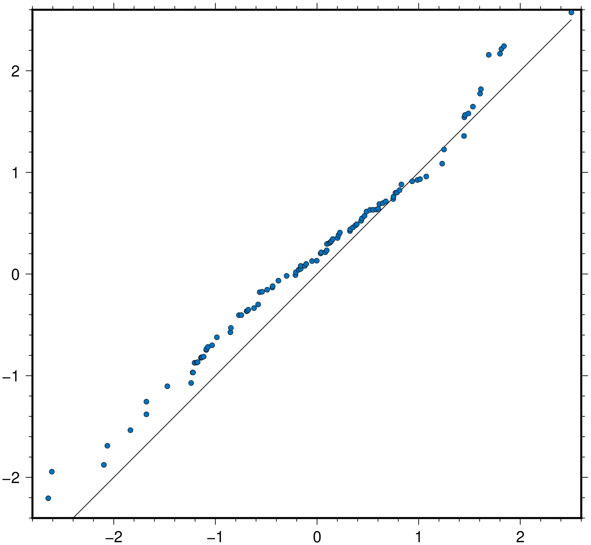
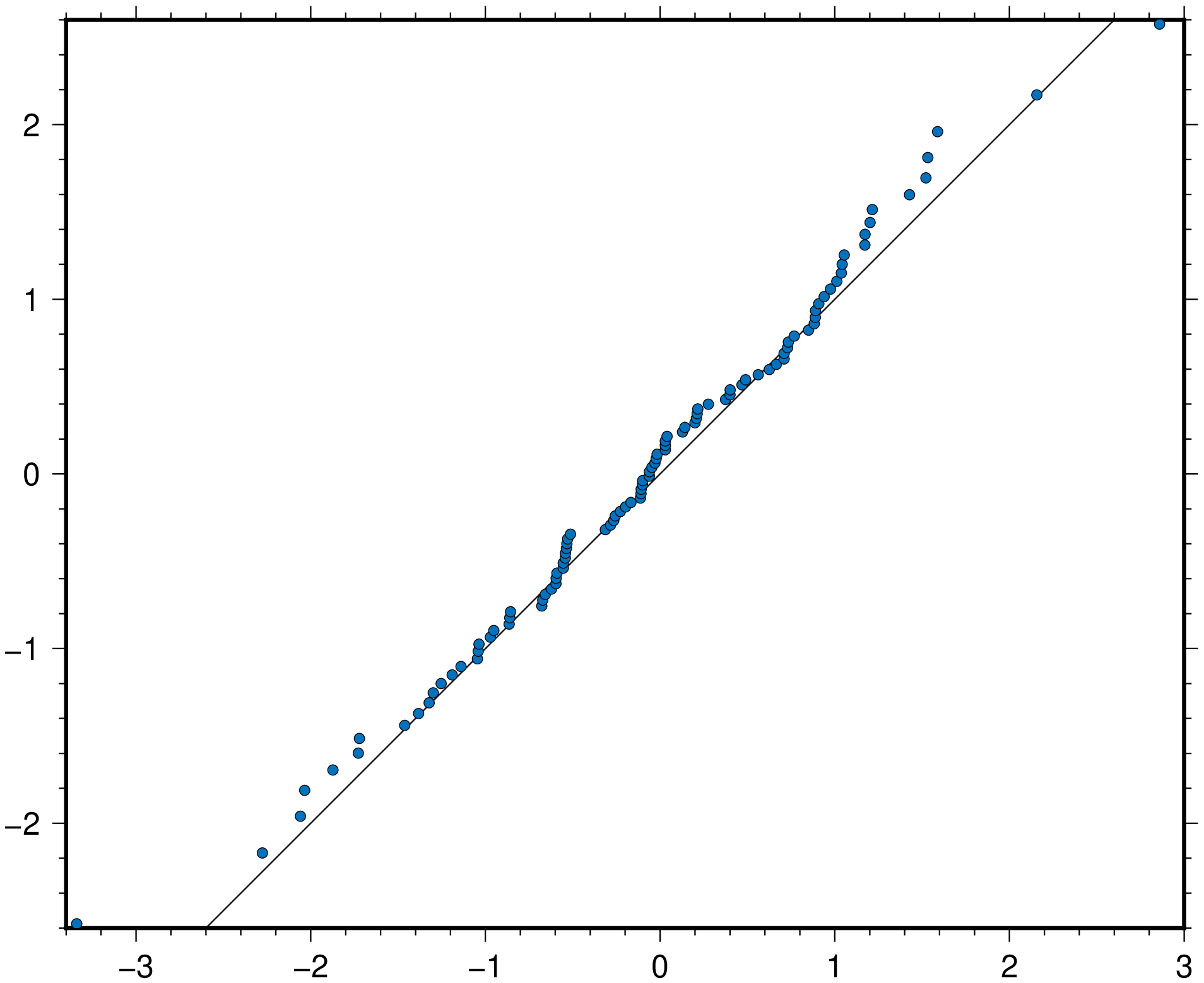
The qqplot function compares the quantiles of two distributions. The qqnorm is a shorthand for comparing a distribution to the normal distribution. If the distributions are similar the points will be on a straight line.
qqplot(x,y, ...) displays a quantile-quantile plot of the quantiles of the sample data x versus the quantiles of the sample data y. If the samples come from the same distribution, then the plot appears linear.
qqplot(x, ...) displays a quantile-quantile plot of the quantiles of the sample data x versus the theoretical quantile values from a normal distribution. If the distribution of x is normal, then the data plot appears linear. A common used alias to this form is the qqnorm function.
This module is a subset of plot to make it simpler to draw stair plots. So not all (fine) controlling parameters are not listed here. For the finest control, user should consult the plot module.
Parameters
qqline : – Determines how to compute a fit line for the Q-Q plot. The options are
-identity: draw the line y = x (the deafult).fit: draw a least squares line fit of the quantile pairs.fitrobustorquantile: draw the line that passes through the first and third quartiles of the distributions.none: do not draw any line.
Broadly speaking, qqline=:identity is useful to see if x and y follow the same distribution, whereas qqline=:fit and qqline=:fitrobust are useful to see if the distribution of y can be obtained from the distribution of x via an affine transformation.
For fine the lines settings use the same options as in the plot module. Nemely
lworltfor controling the line thickness,lcfor line color,lsfor line styles, etc...
B or axes or frame
Set map boundary frame and axes attributes. Default is to draw and annotate left, bottom and vertical axes and just draw left and top axes. More at frame
J or proj or projection : – proj=<parameters>
Select map projection. More at proj
R or region or limits : – limits=(xmin, xmax, ymin, ymax) | limits=(BB=(xmin, xmax, ymin, ymax),) | limits=(LLUR=(xmin, xmax, ymin, ymax),units="unit") | ...more
Specify the region of interest. More at limits. For perspective view view, optionally add zmin,zmax. This option may be used to indicate the range used for the 3-D axes. You may ask for a larger w/e/s/n region to have more room between the image and the axes.
G or markerfacecolor or MarkerFaceColor or markercolor or mc or fill
Select color or pattern for filling of symbols [Default is no fill]. Note that plot will search for fill and pen settings in all the segment headers (when passing a GMTdaset or file of a multi-segment dataset) and let any values thus found over-ride the command line settings (but those must be provided in the terse GMT syntax). See Setting color for extend color selection (including color map generation).
W or pen=
pen
Set pen attributes for the arrow stem [Defaults: width = default, color = black, style = solid]. See Pen attributes and Vector attributes for arrow line terminations.
U or time_stamp : – time_stamp=true | time_stamp=(just="code", pos=(dx,dy), label="label", com=true)
Draw GMT time stamp logo on plot. More at timestamp
V or verbose : – verbose=true | verbose=level
Select verbosity level. More at verbose
X or xshift or x_offset : xshift=true | xshift=x-shift | xshift=(shift=x-shift, mov="a|c|f|r")
Shift plot origin. More at xshift
Y or yshift or y_offset : yshift=true | yshift=y-shift | yshift=(shift=y-shift, mov="a|c|f|r")
Shift plot origin. More at yshift
figname or savefig or name : – figname=
name.png
Save the figure with thefigname=name.extwhereextchooses the figure image format.
Examples
using GMT
qqplot(randn(100), randn(100), show=true)
using GMT
qqplot(randn(100), show=true)
These docs were autogenerated using GMT: v1.23.0