radar

radar(cmd0="", arg1=nothing; axeslimts=Float64[], annotall=false, axeslabels=String[], kwargs...)

keywords: GMT, Julia, radar plots

Radar plots are a useful way for seeing which variables have similar values or if there are outliers amongst each variable. By default we expect a matrix, or a GMTdatset (or a vector of them) with normalized values. This is so because a radar plot has multiple axis that each have different limits. So the options are to pass normalized variables or set each axis limits via the axeslimts option.

radar(A, ...) plots the elements in the rows of A if it is a mtrix creating a polygon per row, or just one polygon if A is a vector.

This module is a subset of plot to make it simpler to draw stair plots. So not all (fine) controlling parameters are not listed here. For the finest control, user should consult the plot module.

Parameters

• axeslabels or labels : – axeslabels=["??","??",...] | labels=["??","??",...]
  String vector with the names of each variable axis. Plot a default "Label?" if not provided..

• axeslimts : – axeslimts=[...]
  A vector with the same size as columns in the input matrix with the max extent of each variable. NOTE that if you don't provide this option we assume input data is normalized.

• annotall : – annotall=true
  By default only the first axis is annotated, which is all it needs when variables are normalized. However, when using non-normalized variables it may be useful to show the limits of each axis.

By default the polygons are not filled but that is often not so nice. To fill with the default cyclic color use just fill=true. Other options are to use:

• fill or fillcolor : – fill=true | fill=["color1", "color2", ...]*\ A string vector with polygon colors. If number of colors is less then number of polygons we cycle through the number of provided colors.

• fillalpha : – fillalpha=[0.5, 0.7, ...]
  The default is to paint polygons with a transparency of 70%. For other transparency values pass in a vector of transparencies (between [0-1] or ]1-100]) via this option.

• For fine the lines settings use the same options as in the plot module. Nemely lw or lt for controling the line thickness, lc for line color, ls for line styles, etc...

• B or axes or frame
  Set map boundary frame and axes attributes. Default is to draw and annotate left, bottom and vertical axes and just draw left and top axes. More at frame

• J or proj or projection : – proj=<parameters>
  Select map projection. More at proj

• R or region or limits : – limits=(xmin, xmax, ymin, ymax) | limits=(BB=(xmin, xmax, ymin, ymax),) | limits=(LLUR=(xmin, xmax, ymin, ymax),units="unit") | ...more
  Specify the region of interest. More at limits. For perspective view view, optionally add zmin,zmax. This option may be used to indicate the range used for the 3-D axes. You may ask for a larger w/e/s/n region to have more room between the image and the axes.

• G or markerfacecolor or MarkerFaceColor or markercolor or mc or fill
  Select color or pattern for filling of symbols [Default is no fill]. Note that plot will search for fill and pen settings in all the segment headers (when passing a GMTdaset or file of a multi-segment dataset) and let any values thus found over-ride the command line settings (but those must be provided in the terse GMT syntax). See Setting color for extend color selection (including color map generation).

• W or pen=pen
  Set pen attributes for the arrow stem [Defaults: width = default, color = black, style = solid]. See Pen attributes

• U or time_stamp : – time_stamp=true | time_stamp=(just="code", pos=(dx,dy), label="label", com=true)
  Draw GMT time stamp logo on plot. More at timestamp

• V or verbose : – verbose=true | verbose=level
  Select verbosity level. More at verbose

• X or xshift or x_offset : xshift=true | xshift=x-shift | xshift=(shift=x-shift, mov="a|c|f|r")
  Shift plot origin. More at xshift

• Y or yshift or y_offset : yshift=true | yshift=y-shift | yshift=(shift=y-shift, mov="a|c|f|r")
  Shift plot origin. More at yshift

• figname or savefig or name : – figname=name.png
  Save the figure with the figname=name.ext where ext chooses the figure image format.

Examples

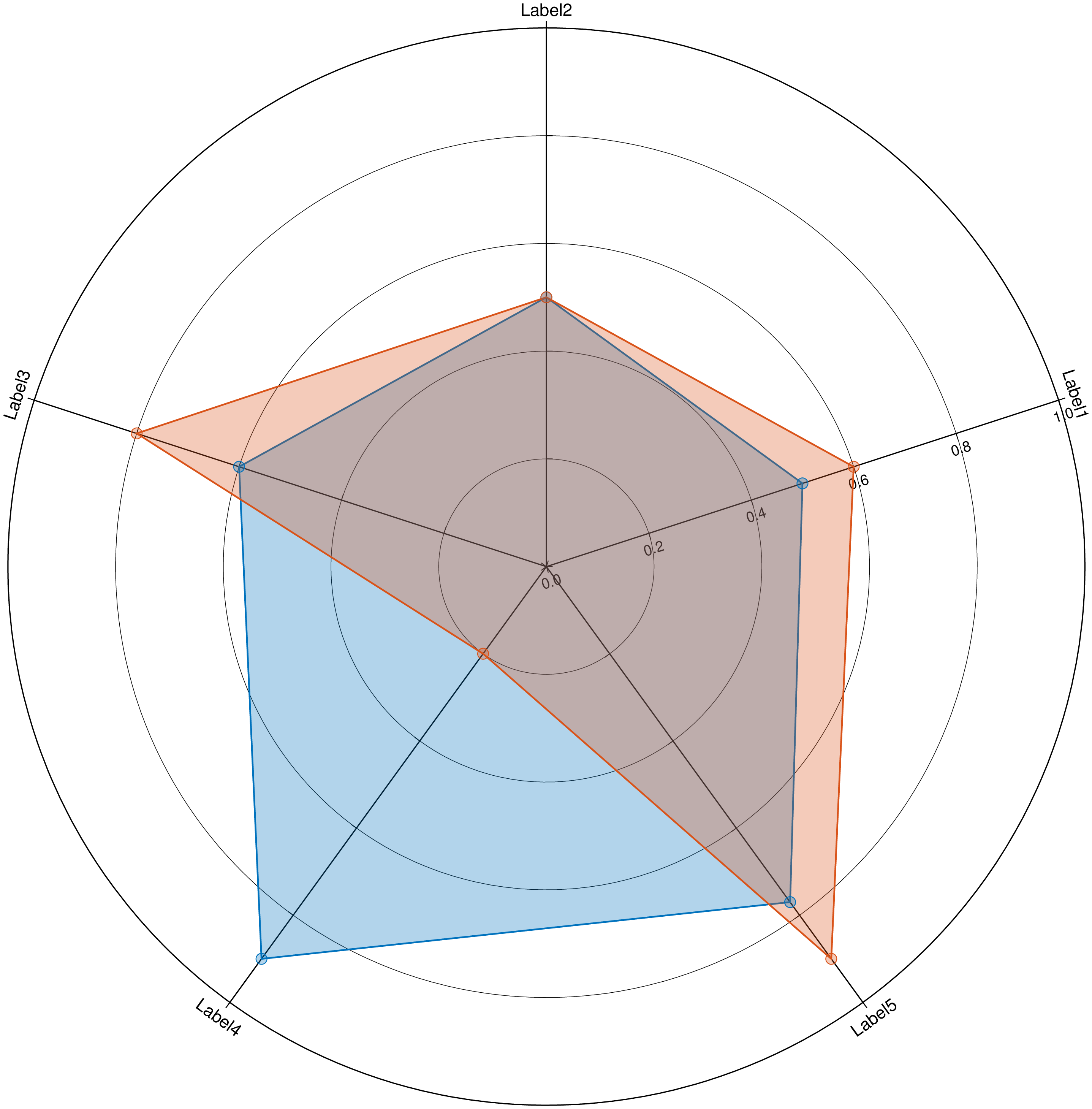
Create a

using GMT
radar([0.5 0.5 0.6 0.9 0.77; 0.6 0.5 0.8 0.2 0.9], show=true, marker=:circ, fill=true)

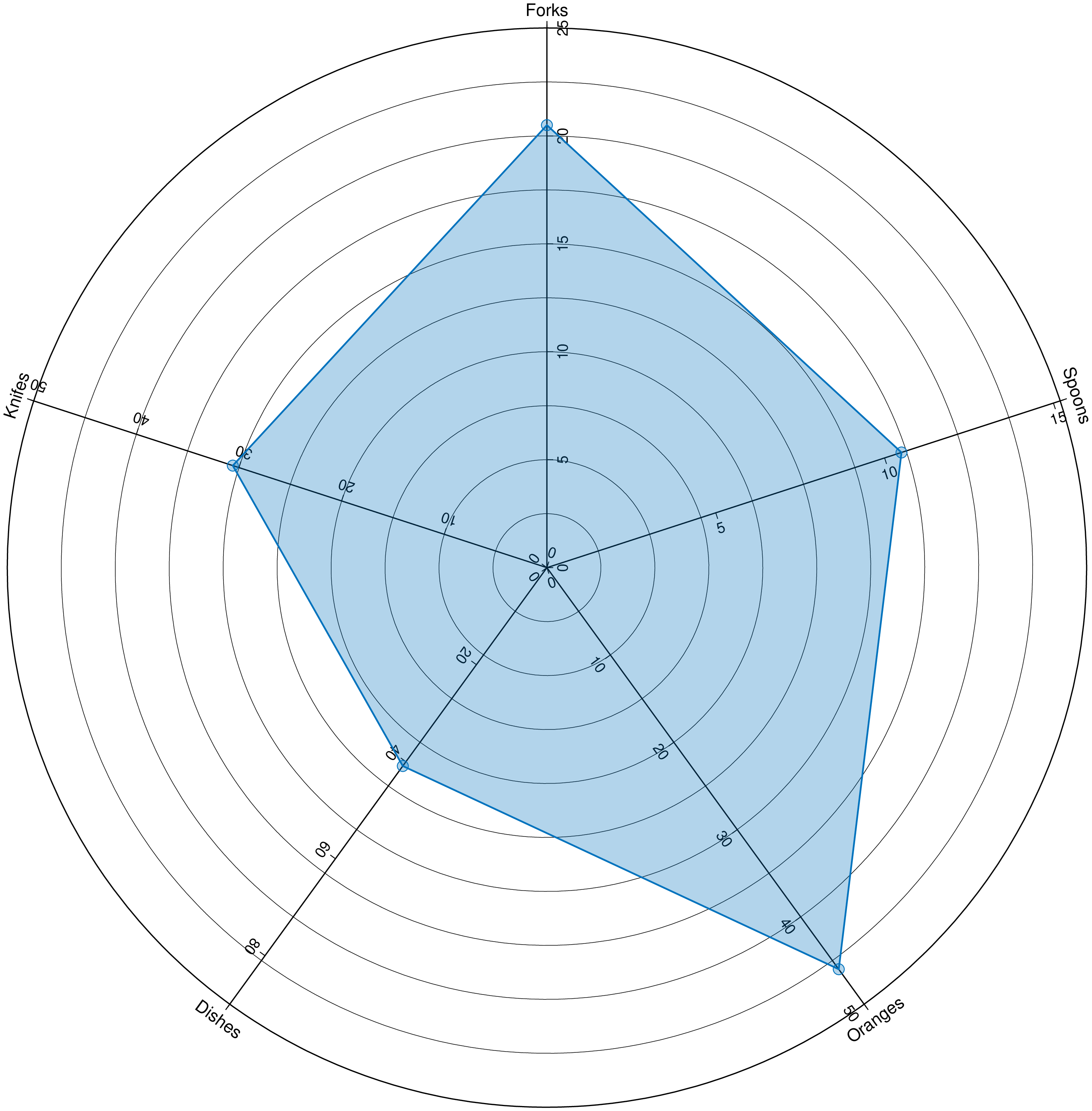
Plot

using GMT
radar([10.5 20.5 30.6 40.9 46], axeslimts=[15, 25, 50, 90, 50], annotall=true, marker=:circ, fill=true, 
      labels=["Spoons","Forks","Knifes","Dishes","Oranges"], show=1)