sample1d

sample1d(cmd0::String="", arg1=nothing, kwargs...)

keywords: GMT, Julia, resample

Resample 1-D table data using splines

Description

Reads a multi-column data set and interpolates the time-series or spatial profile at locations where the user needs the values. The user must provide the column number of the independent (monotonically increasing or decreasing) variable, here called time (it may of course be any type of quantity) when that is not the first column in data set. Equidistant or arbitrary sampling can be selected. All columns are resampled based on the new sampling interval. Several interpolation schemes are available, in addition to a smoothing spline which trades off misfit for curvature. Extrapolation outside the range of the input data is not supported.

Required Arguments

table
One or more data tables containing the independent time variable (which must be monotonically in/de-creasing) and any number of optional columns holding other data values.

Optional Arguments

A or resample : – resample="f|p|m|r|R" | resample="f|p|m|r|R[+d][+l]"
For track resampling (if inc...unit is set) we can select how this is to be performed. Use resample=:f to keep original points, but add intermediate points if needed; note this selection does not necessarily yield equidistant points [Default]. resample=:m as f but first follow meridian (along y) then parallel (along x). p as f but first follow parallel (along y) then meridian (along x). r to resample at equidistant locations; input points are not necessarily included in the output. R as r but adjust given spacing to fit the track length exactly. Finally, append +d to delete duplicate input records (identified by having no change in the time column, and +l if distances should be measured along rhumb lines (loxodromes)). Note: Calculation made for loxodromes is spherical, hence spherical=:ellipsoidal cannot be used in combination with +l.

E or keeptext : – keeptext=true
If the input dataset contains records with trailing text then we will attempt to add these to output records that exactly match the input times. Output records that have no matching input record times will have no trailing text appended [Default ignores trailing text]. Needs GMT6.4 or higher.

F or interp : – interp=type | interp=(type, [,par], "derivative")
The default is Akima. You may change the default interpolant; see GMT_INTERPOLANT in your gmt.conf file.

Choose type from (the *interp_type=type* form): - **l**inear - **a**kima spline - **c**ubic (natural cubic spline) - **n**ointerp (no interpolation: nearest point) - **s**moothing cubic spline; append fit parameter *p*. Note, in this case one must pass only the first char, the **s** and the fitting parameter. Example: **interp="s0.01"** You may optionally evaluate the first or second derivative of the spline by appending **+d1** or **+d2**, respectively. When using the second form (the *interp_type=(...)*), the first member is the same as above, except the smooth and the derivatives. To select first or second derivative use the :first or :second keywords. Examples of this syntax: **interp=(:akima, :first)**, or **interp=(:smoothing, 0.1)**, or **interp=(:smoothing, 0.1, :second)**.

using GMT
mat = [0 0; 1 1; 2 1.5; 3 1.25; 4 1.5; 4.5 3; 5 2; 6 2.5];
gmtbegin()
    D = sample1d(mat, inc=0.01, interp=:cubic);
    plot(D, region=(-0.1,6.1,-0.1,3.1), figsize=(14,6), xlabel=:u, ylabel="u(x)", lw=1, legend="Cubic spline (F=:c)")
    D = sample1d(mat, inc=0.01, interp=(:smooth, 1));
    plot!(D, lw=1, lc=:orange, legend="Smooth cubic spline (F=:s1)")
    D = sample1d(mat, inc=0.01, interp=:linear);
    plot!(D, lw=1, lc=:blue, legend="Linear spline (F=:l)")
    D = sample1d(mat, inc=0.01, interp=:akima);
    plot!(D, lw=1, lc=:red, legend="Akima spline (F=:a)")
    D = sample1d(mat, inc=0.01, interp=:nointerp);
    plot!(D, lw=1, lc=:darkgreen, legend="Nearest neighbor (F=:n)")
    plot!(mat, marker=:circ, ms=0.25, mc=:red, ml=:thin, legend="Data")
    legend(position=(inside=:TL, width=4.9, offset=0.2), box=(pen=1, fill=:white, shaded=true))
gmtend(:show)

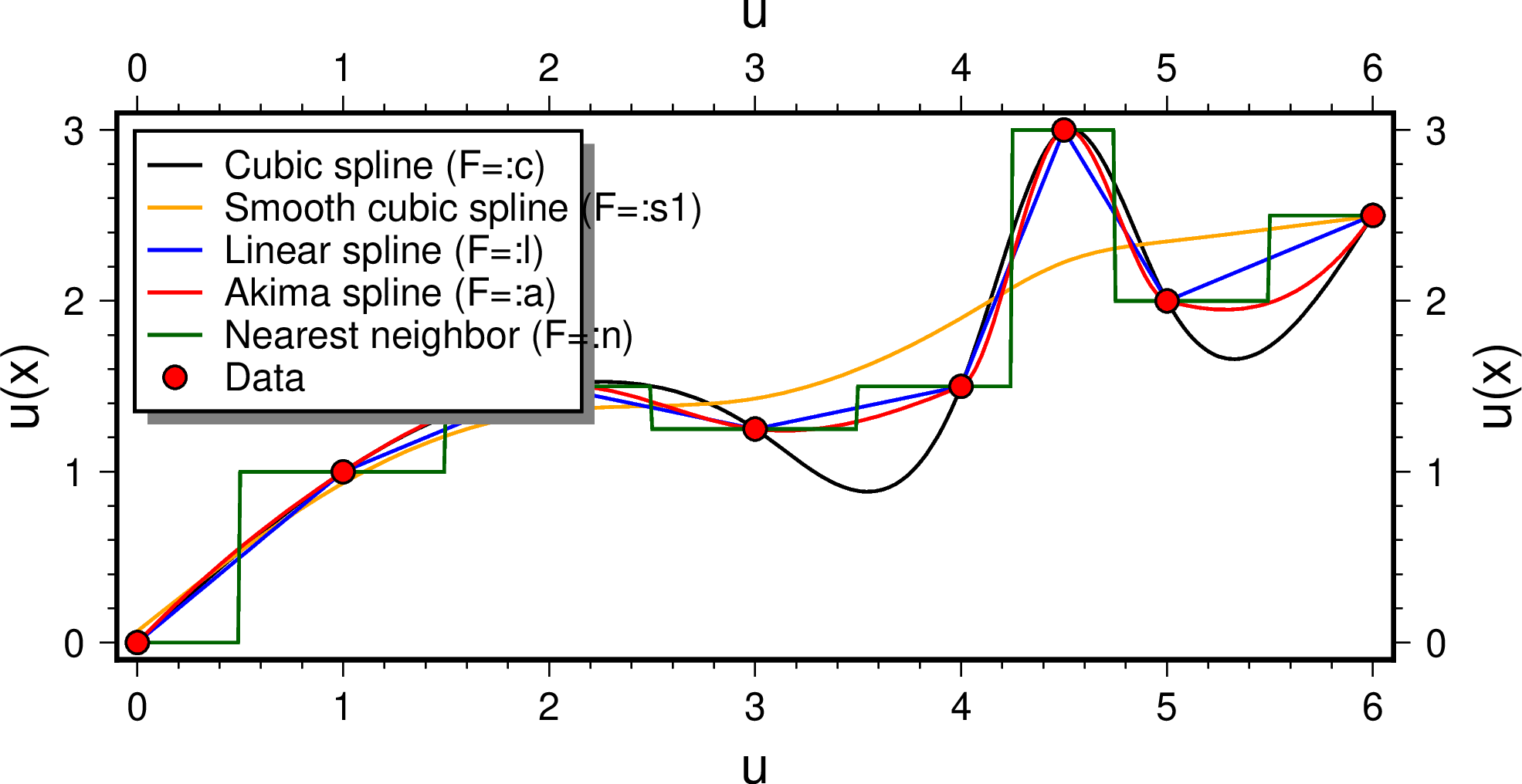
The interp option lets you choose among several interpolators, including one that is approximate (the smoothing spline). You can also specify that you actually need a derivative of the solution instead of the value.

N or time_col or timecol : – timecol=t_col
Sets the column number of the independent time variable [Default is 0 (first)].

T or range or inc : – range=(min,max,inc[,:number,:log2,:log10]) | range=[list] | range=file
Make evenly spaced time-steps from min to max by inc [Default uses input times]. The form range=list means a online list of time coordinates like for example: range=[13,15,16,22.5] whilst range=file means: read the time coordinates from file, one coordinate per row in file. Note: For resampling of spatial (x,y or lon,lat) series you must give an increment with a valid distance unit; see Units for map units or use c if plain Cartesian coordinates. The first two columns must contain the spatial coordinates. From these we calculate distances in the chosen units and interpolate using this parametric series.

cumdist or cumsum : – cumdist=true
Compute the cumulative distance along the input line. Note that for this the first two columns must contain the spatial coordinates and the accumulated distance is appended after last column of the table.

V or verbose : – verbose=true | verbose=level
Select verbosity level. More at verbose

W or weights : – weights=col
Sets the column number of the weights to be used with a smoothing cubic spline. Requires interp=:s.

bi or binary_in : – binary_in=??
Select native binary format for primary table input. More at

bo or binary_out : – binary_out=??
Select native binary format for table output. More at

di or nodata_in : – nodata_in=??
Substitute specific values with NaN. More at

e or pattern : – pattern=??
Only accept ASCII data records that contain the specified pattern. More at

f or colinfo : – colinfo=??
Specify the data types of input and/or output columns (time or geographical data). More at

g or gap : – gap=??
Examine the spacing between consecutive data points in order to impose breaks in the line. More at

h or header : – header=??
Specify that input and/or output file(s) have n header records. More at

i or incol or incols : – incol=col_num | incol="opts"
Select input columns and transformations (0 is first column, t is trailing text, append word to read one word only). More at incol

j or metric or spherical_dist or spherical : – metric=greatcirc or spherical=:flat or spherical=:ellipsoidal
Determine how spherical distances are calculated in modules that support this [Default is spherical=:greatcirc]. GMT has different ways to compute distances on planetary bodies:

- spherical=:greatcirc to perform great circle distance calculations, with parameters such as distance increments or radii compared against calculated great circle distances [Default is spherical=:greatcirc]. - spherical=:flat to select Flat Earth mode, which gives a more approximate but faster result. - spherical=:ellipsoidal to select ellipsoidal (or geodesic) mode for the highest precision and slowest calculation time. Note: All spherical distance calculations depend on the current ellipsoid (PROJ_ELLIPSOID), the definition of the mean radius (PROJ_MEAN_RADIUS), and the specification of latitude type (PROJ_AUX_LATITUDE). Geodesic distance calculations is also controlled by method (PROJ_GEODESIC).

o or outcol : – outcol=??
Select specific data columns for primary output, in arbitrary order. More at

q or inrows : – inrows=??
Select specific data rows to be read and/or written. More at

w or wrap or cyclic : – wrap=??
Convert input records to a cyclical coordinate. More at

s or skiprows or skip_NaN : – skip_NaN=true | skip_NaN="<cols[+a][+r]>"
Suppress output of data records whose z-value(s) equal NaN. More at

Units

For map distance unit, append unit d for arc degree, m for arc minute, and s for arc second, or e for meter [Default unless stated otherwise], f for foot, k for km, M for statute mile, n for nautical mile, and u for US survey foot. By default we compute such distances using a spherical approximation with great circles (-jg) using the authalic radius (see PROJ_MEAN_RADIUS). You can use -jf to perform “Flat Earth” calculations (quicker but less accurate) or -je to perform exact geodesic calculations (slower but more accurate; see PROJ_GEODESIC for method used).

Notes

The smoothing spline s(t) requires a fit parameter p that allows for the trade-off between an exact interpolation (fitting the data exactly; large p) to minimizing curvature (p approaching 0). Specifically, we seek to minimize

\[ F_p (s)= K (s) + p E (s), \quad p > 0 \]

where the misfit is evaluated as

\[ E (s)= \sum^n_{i=1} \left [ \frac{s(t_i) - y_i}{\sigma_i} \right ]^2 \]

and the curvature is given by the integral over the domain of the second derivative of the spline

\[ K (s) = \int ^b _a [s''(t) ]^2 dt. \]

Trial and error may be needed to select a suitable p.

Examples

To resample the file profiles.tdgmb, which contains (time,distance,gravity,magnetics,bathymetry) records, at 1 km equidistant intervals using Akima's spline, use:

D = sample1d("profiles.tdgmb", timecol=1, interp=:akima, inc=1)

To resample the file depths.dt at positions listed in the file grav_pos.dg, using a cubic spline for the interpolation, use:

D = sample1d("depths.txt", range="grav_pos.dg", interp=:cubic)

To resample the file points.txt every 0.01 from 0-6, using a cubic spline for the interpolation, but output the first derivative instead (the slope), try:

Ds = sample1d("points.txt", range=(0,6,0.01), interp=(cubic, :first))

To resample the file track.txt which contains lon, lat, depth every 2 nautical miles, use:

D = sample1d("track.txt", inc="2n", resample=:R)

To do approximately the same, but make sure the original points are included, use:

D = sample1d("track.txt", inc="2n", resample=:f)

To obtain a rhumb line (loxodrome) sampled every 5 km instead, use:

D = sample1d("track.txt", inc="5k", resample="R+l")

To sample temperatures.txt every month from 2000 to 2018, use

Dmo = sample1d("temperatures.txt", range=("2000T", "2018T", "1o"))

To use a smoothing spline on a topographic profile for a given fit parameter, try:

sample1d("@topo_crossection.txt", range(300,500,0.1), interp=(:smooth, 0.001))