stem

stem(cmd0::String="", arg1=nothing; kwargs...)

keywords: GMT, Julia, stem plots

Reads (x,y) pairs and plot the data sequence, y, as stems that extend from a baseline along the x-axis. The data values are indicated by circles terminating each stem. The input can either be a file name of a file with at least two columns (x,y), but optionally more, a GMTdatset object with also two or more columns, or direct x,y inputs

stem(x,y, ...) plots the elements in y at the locations specified by x. The inputs x,y can be vectors or a vector and a matrix, both with the same number of rows.

stem(D::GMTdatset, yvar, ...) plots the specified variable from the GMTdatset against the row indices of the table. To plot one set of y-values, specify one variable for yvar. This can take the form of column names or column numbers. To plot multiple sets of y-values, specify multiple variables for yvar. Example yvar=:Y or yvar=(2,3), or yvar=[:Y, :Z1, :Z2].

stem(D::GMTdatset,xvar,yvar) plots the variables xvar and yvar from the table D. You can specify one or multiple variables for yvar and one only for xvar.

This module is a subset of plot to make it simpler to draw stem plots. So not all (fine) controlling parameters are not listed here. For the finest control, user should consult the plot module.

Parameters

• multicol : – multicol=true
  Use this option when passing a multicolumn input and and plot a stemplot for each column.

• nobaseline : – nobaseline=true
  If nobaseline=true do not paint the horizontal baseline from which the stems start.

• B or axes or frame
  Set map boundary frame and axes attributes. Default is to draw and annotate left, bottom and vertical axes and just draw left and top axes. More at frame

• J or proj or projection : – proj=<parameters>
  Select map projection. More at proj

• R or region or limits : – limits=(xmin, xmax, ymin, ymax) | limits=(BB=(xmin, xmax, ymin, ymax),) | limits=(LLUR=(xmin, xmax, ymin, ymax),units="unit") | ...more
  Specify the region of interest. More at limits. For perspective view view, optionally add zmin,zmax. This option may be used to indicate the range used for the 3-D axes. You may ask for a larger w/e/s/n region to have more room between the image and the axes.

• G or markerfacecolor or MarkerFaceColor or markercolor or mc or fill
  Select color or pattern for filling of symbols [Default is no fill]. Note that plot will search for fill and pen settings in all the segment headers (when passing a GMTdaset or file of a multi-segment dataset) and let any values thus found over-ride the command line settings (but those must be provided in the terse GMT syntax). See Setting color for extend color selection (including color map generation).

• W or pen=pen
  Set pen attributes for the arrow stem [Defaults: width = default, color = black, style = solid]. See Pen attributes

• U or time_stamp : – time_stamp=true | time_stamp=(just="code", pos=(dx,dy), label="label", com=true)
  Draw GMT time stamp logo on plot. More at timestamp

• V or verbose : – verbose=true | verbose=level
  Select verbosity level. More at verbose

• X or xshift or x_offset : xshift=true | xshift=x-shift | xshift=(shift=x-shift, mov="a|c|f|r")
  Shift plot origin. More at xshift

• Y or yshift or y_offset : yshift=true | yshift=y-shift | yshift=(shift=y-shift, mov="a|c|f|r")
  Shift plot origin. More at yshift

• figname or savefig or name : – figname=name.png
  Save the figure with the figname=name.ext where ext chooses the figure image format.

Examples

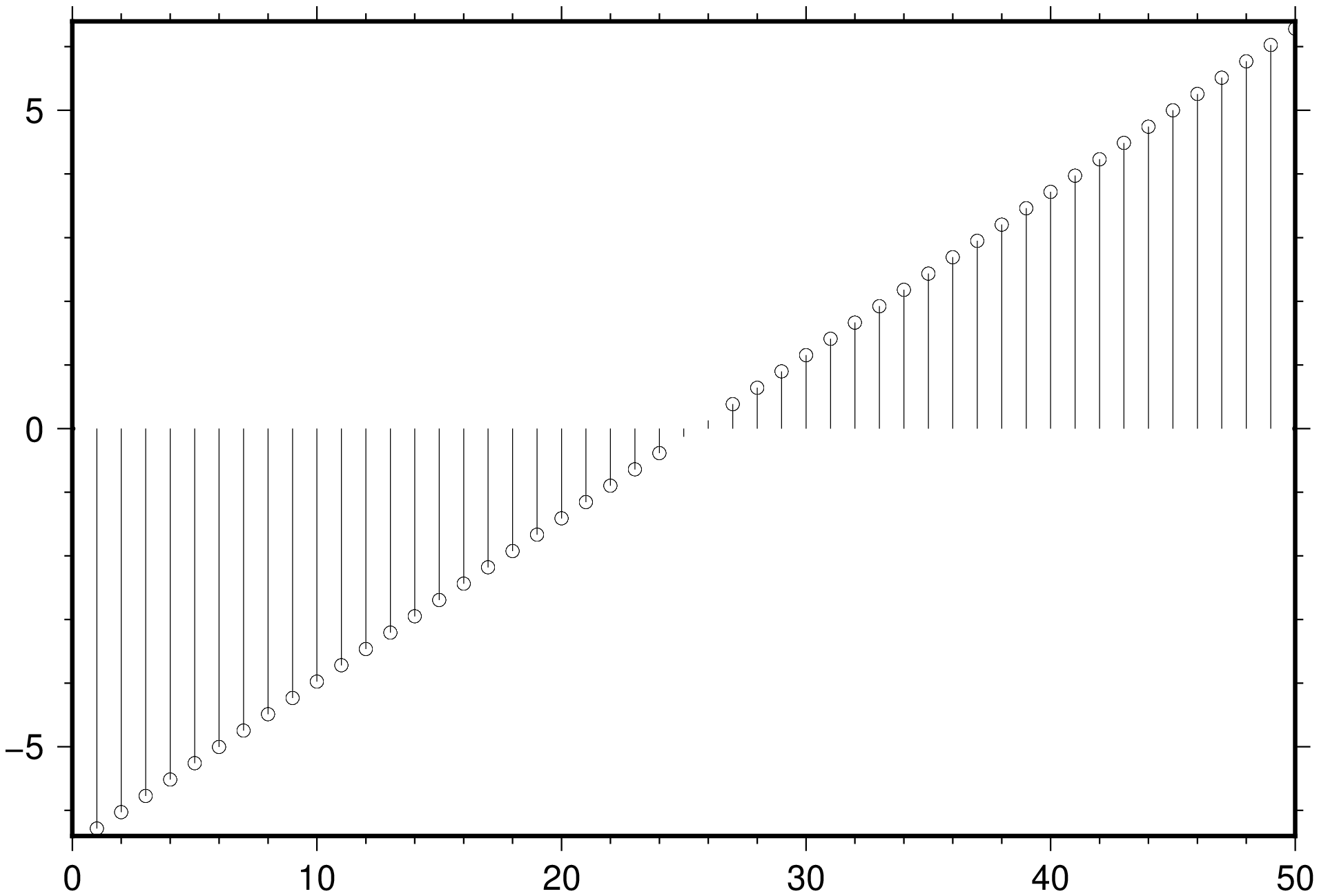
Create a stem plot of 50 data values between −2π and 2π.

using GMT
Y = linspace(-2*pi,2*pi,50);
stem(Y, show=true)

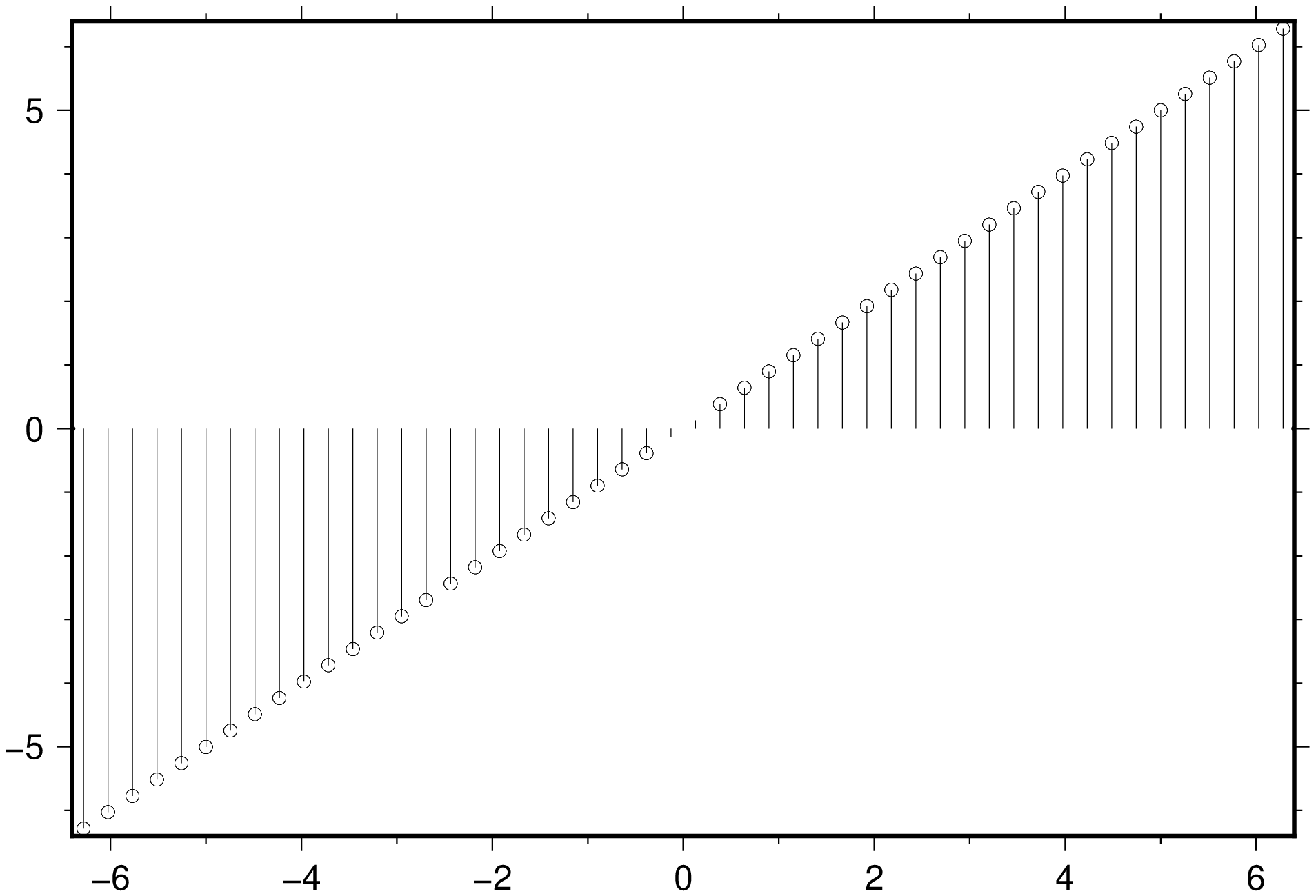
The same but now specify the set of x values for the stem plot.

using GMT
Y = linspace(-2*pi,2*pi,50);
stem([Y Y], show=true)

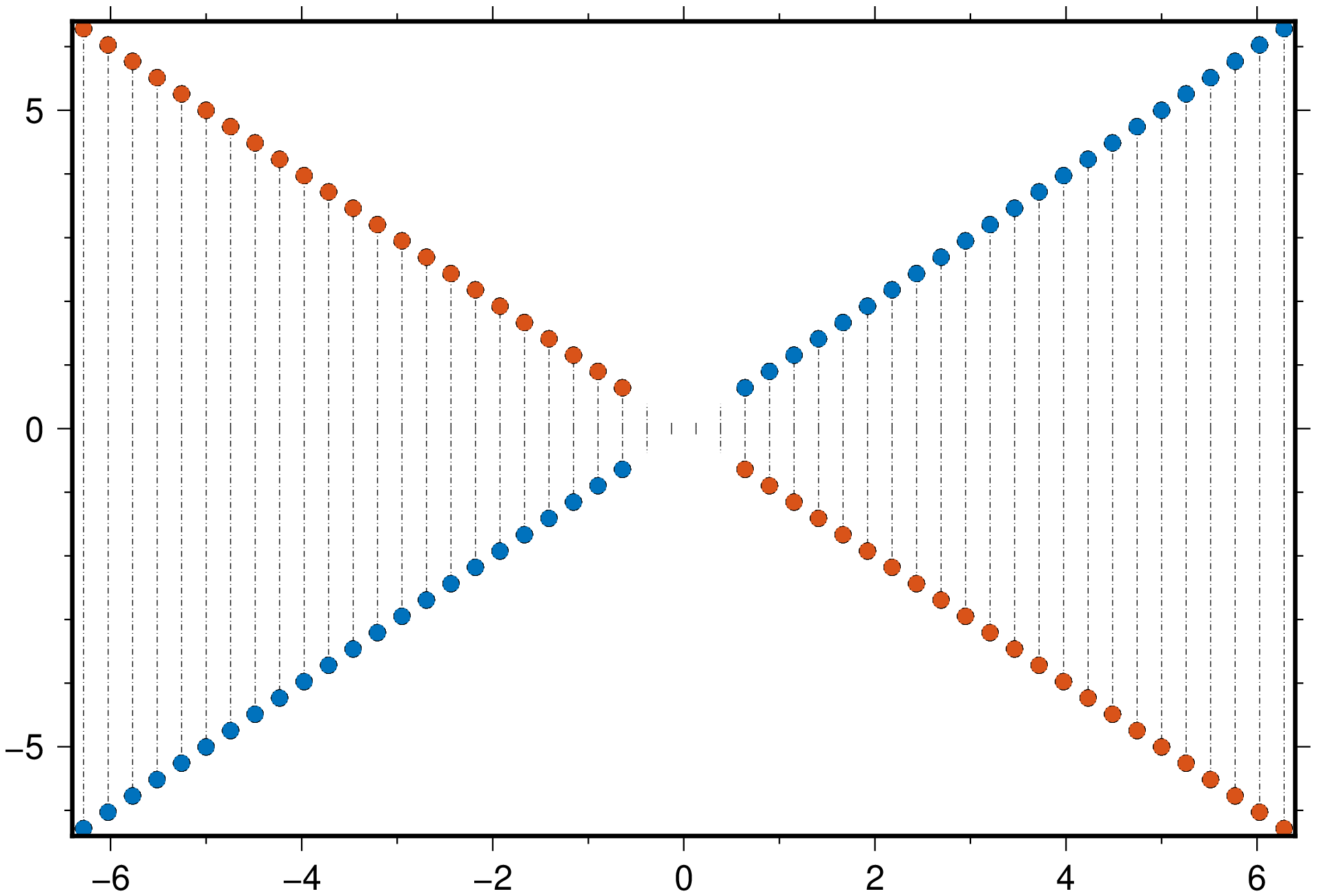
Two of them and with some variations.

using GMT
Y = linspace(-2*pi,2*pi,50);
stem(Y,[Y -Y], multicol=true, fill=true, ms="10p", nobaseline=true, ls=:DashDot, show=true)