wiggle
wiggle(cmd0::String="", arg1=nothing; kwargs...)Plot z = f(x,y) anomalies along tracks
Description
Reads (x, y,z) triplets from file or table and plots z as a function of distance along track. This means that two consecutive (x, y) points define the local distance axis, and the local z axis is then perpendicular to the distance axis, forming a right-handed coordinate system. The user may set a preferred positive anomaly plot direction, and if the positive normal is outside the ±90 degree window around the preferred direction, then 180 degrees are added to the direction. Either the positive or the negative wiggle (or both) may be shaded.
Required Arguments
table
One or more data tables holding a number of data columns.
J or proj or projection : – proj=<parameters>
Select map projection. More at proj
R or region or limits : – limits=(xmin, xmax, ymin, ymax) | limits=(BB=(xmin, xmax, ymin, ymax),) | limits=(LLUR=(xmin, xmax, ymin, ymax),units="unit") | ...more
Specify the region of interest. More at limits. For perspective view view, optionally add zmin,zmax. This option may be used to indicate the range used for the 3-D axes. You may ask for a larger w/e/s/n region to have more room between the image and the axes.
R or region or limits : – limits=(xmin, xmax, ymin, ymax, zmin, zmax) | limits=(BB=(xmin, xmax, ymin, ymax, zmin, zmax),) | ...more
Specify the region of interest. Default limits are computed from data extents. More at limits
Z or ampscale or amp_scale : – ampscale=??
Gives anomaly scale in data-units/distance-unit. Append c, i, or p to indicate the distance unit (cm, inch, or point); if no unit is given we use the default unit that is controlled byPROJ_LENGTH_UNIT.
Optional Arguments
A azimuth : – azimuth=az
Sets the preferred positive azimuth. Positive wiggles will "gravitate" towards that direction, i.e., azimuths of the normal direction to the track will be flipped into the -90/+90 degree window centered on azimuth and that defines the positive wiggle side. If no azimuth is given the no preferred azimuth is enforced.
B or axes or frame
Set map boundary frame and axes attributes. Default is to draw and annotate left, bottom and vertical axes and just draw left and top axes. More at frame
C or center : – center=??
Subtract center from the data set before plotting [0].
D or scale_bar : – pos=(map=(lon,lat), inside=true, outside=true, norm=(x,y), paper=(x,y), justify=code, offset=XX, anchor=XX, label="the-label", label_left=true)
Defines the reference point on the map for the vertical scale bar using one of four coordinate systems: (1) Use map=true for map (user) coordinates, (2) use inside=true or outside=true (the default) for setting anchor via a 2-char justification code that refers to the (invisible) map domain rectangle, (3) use norm=true for normalized (0-1) coordinates, or (4) use paper=true for plot coordinates (inches, cm, etc.). All but paper=true requires both region and proj to be specified.
Use width=(width,height) to set the *length* (and *height*) of the scale bar in data (*z*) units.
By default, the anchor point on the legend is assumed to be the bottom left corner (:ML), but this
can be changed by appending justify followed by a 2-char justification code *justify* (see text).
**Note**: If inside is used (the default) then *justify* defaults to the same as refpoint,
if outside is used then justify defaults to the mirror opposite of refpoint.
Move scale label to the left side with label_left=true [Default is to the right of the scale].
Use label="The label" to set the *z* unit label that is used in the scale label [no unit].
The FONT_ANNOT_PRIMARY is used for the font setting, while MAP_TICK_PEN_PRIMARY
is used to draw the scale bar.
W or pen=
pen
Set pen attributes for the arrow stem [Defaults: width = default, color = black, style = solid]. See Pen attributes and Vector attributes for arrow line terminations.
G or fill : – fill=fill[+n][+p]
Set fill shade, color or pattern for positive and/or negative wiggles [Default is no fill]. Optionally, append +p to fill positive areas (this is the default behavior). Append +n to fill negative areas. Append +n+p to fill both positive and negative areas with the same fill. Note: You will need to repeat this option to select different fills for the positive and negative wiggles, but sie we cannot repeat keywords the solution is to pass in a tuple of tuples or of NamedTuples. For simpler cases one can pass also a 2 elements vector of strings thet will be used as is, that is, without any further parsing. See example below.
I or fixed_azim : fixed_azim=az
Set a fixed azimuth projection for wiggles [Default uses track azimuth, but see |-A|]. With this option, the calculated track-normal azimuths are overridden by fixed_az.
T or track : – track=pen
Draw track [Default is no track]. Append pen attributes to use [Defaults: width = 0.25p, color = black, style = solid].
U or time_stamp : – time_stamp=true | time_stamp=(just="code", pos=(dx,dy), label="label", com=true)
Draw GMT time stamp logo on plot. More at timestamp
V or verbose : – verbose=true | verbose=level
Select verbosity level. More at verbose
X or xshift or x_offset : xshift=true | xshift=x-shift | xshift=(shift=x-shift, mov="a|c|f|r")
Shift plot origin. More at xshift
Y or yshift or y_offset : yshift=true | yshift=y-shift | yshift=(shift=y-shift, mov="a|c|f|r")
Shift plot origin. More at yshift
bi or binary_in : – binary_in=??
Select native binary format for primary table input. More at
di or nodata_in : – nodata_in=??
Substitute specific values with NaN. More at
e or pattern : – pattern=??
Only accept ASCII data records that contain the specified pattern. More at
f or colinfo : – colinfo=??
Specify the data types of input and/or output columns (time or geographical data). More at
g or gap : – gap=??
Examine the spacing between consecutive data points in order to impose breaks in the line. More at
h or header : – header=??
Specify that input and/or output file(s) have n header records. More at
i or incol or incols : – incol=col_num | incol="opts"
Select input columns and transformations (0 is first column, t is trailing text, append word to read one word only). More at incol
p or view or perspective : – view=(azim, elev)
Default is viewpoint from an azimuth of 200 and elevation of 30 degrees.
Specify the viewpoint in terms of azimuth and elevation. The azimuth is the horizontal rotation about the z-axis as measured in degrees from the positive y-axis. That is, from North. This option is not yet fully expanded. Current alternatives are:view=??
A full GMT compact string with the full set of options.view=(azim,elev)
A two elements tuple with azimuth and elevationview=true
To propagate the viewpoint used in a previous module (makes sense only inbar3!)
More at perspective
q or inrows : – inrows=??
Select specific data rows to be read and/or written. More at
t or transparency or alpha: – alpha=50
Set PDF transparency level for an overlay, in (0-100] percent range. [Default is 0, i.e., opaque]. Works only for the PDF and PNG formats.
w or wrap or cyclic : – wrap=??
Convert input records to a cyclical coordinate. More at
yx : – yx=true
Swap 1st and 2nd column on input and/or output. More at
figname or savefig or name : – figname=
name.png
Save the figure with thefigname=name.extwhereextchooses the figure image format.
Examples
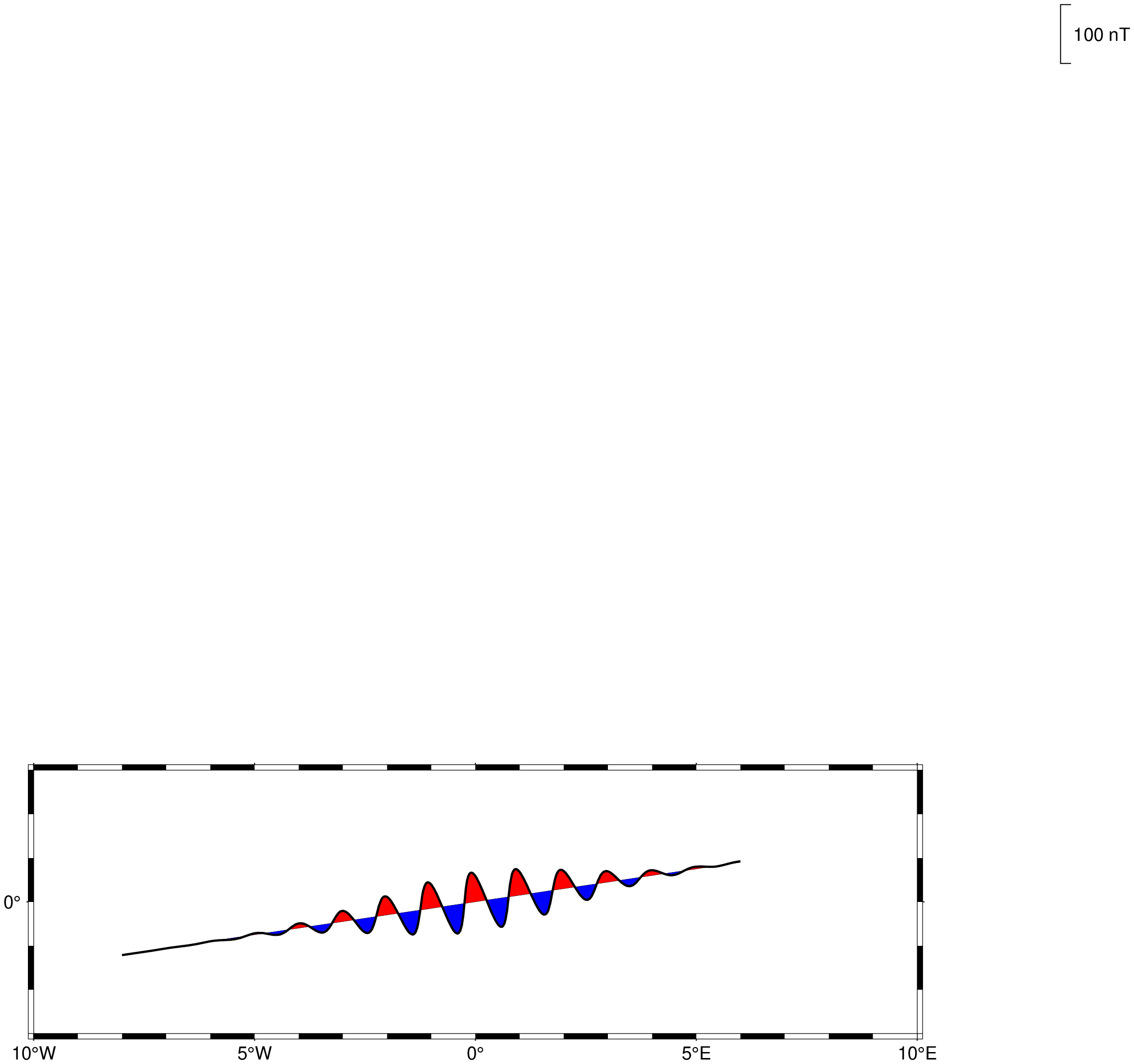
To demonstrate a basic wiggle plot we create some synthetic data with gmtmath and pipe it through wiggle:
using GMT

x = -8:0.01:6;
y = 0.15 .* x;
z = 50 .* exp.(-((x ./ 3) .^ 2)) .* cos.(2pi .* x) .+ y;
wiggle([x y z], region=(-10,10,-3,3), proj=:Merc, ampscale=100,
       scale_bar=(refpoint=:RM, width=100, label=:nT),
       track=:faint, fill=["red+p", "blue+n"], pen=1, show=1)
To plot the magnetic anomaly stored in the file track.xym along track at 500 nTesla/cm (after removing a mean value of 32000 nTesla), using a 15-cm-wide Polar Stereographic map ticked every 5 degrees, with positive anomalies in red on a blue track of width 0.25 points, use
wiggle("track.xym", region=(-20,10,-80,-60), proj=(name=:stere, center=(0,90)),
           ampscale=500, frame=(annot=5,), center=32000, fill=:red, track=(0.25,:blue),
           scale_bar=(refpoint=:RM, width=100, label=:nT), show=1)
and the positive anomalies will in general point in the north direction. We used scale_bar to place a vertical scale bar indicating a 1000 nT anomaly. To instead enforce a fixed azimuth of 45 for the positive wiggles, we add fixed_azim and obtain
wiggle("track.xym", region=(-20,10,-80,-60), proj=(name=:stere, center=(0,90)),
           ampscale=1000, frame=(annot=5,), center=32000, fill=:red, track=(0.25,:blue),
           fixed_azim=45, scale_bar=(refpoint=:RM, width=100, label=:nT), show=1)
See Also
These docs were autogenerated using GMT: v1.33.1