fillsinks

fillsinks(G::GMTgrid; conn=4, region=nothing, saco=false, insitu=false)

keywords: GMT, Julia, fill sinks DTM

Fill sinks in a grid.

This function uses the imfill function to find how to fill sinks in a grid. But since imfill operates on UInt8 matrices only the vertical (z) descrimination of the grid is reduced to 256 levels, which is not that much.

Args

• G::GMTgrid: The input grid to process.

Kwargs

• conn::Int: Connectivity for sink filling (4 or 8). Default is 4.

• region: Limit the action to a region of the grid specified by region. See for example the coast manual for and extended doc on this keword, but note that here only region is accepted and not R, etc...

• saco::Bool: Save the lines (GMTdataset ~contours) used to fill the sinks in a global variable called GMT.SACO. This is intended to avoid return them all the time when function ends. This global variable is a [Dict{String,Union{AbstractArray, Vector{AbstractArray}}}()], so to access its contents you must use:

D = get(GMT.SACO[1], "saco", nothing), where D is now a GMTdataset or a vector of them.

NOTE: It is the user's responsibility to empty this global variable when it is no longer needed.

You do that with: delete!(GMT.SACO[1], "saco")

• insitu::Bool: If true, modify the grid in place. Default is false. Alternatively, use the conventional form fillsinks!(G; conn=4).

Returns

• A new GMTgrid with sinks filled, unless insitu is true, in which case the input grid is modified and returned.

Examples

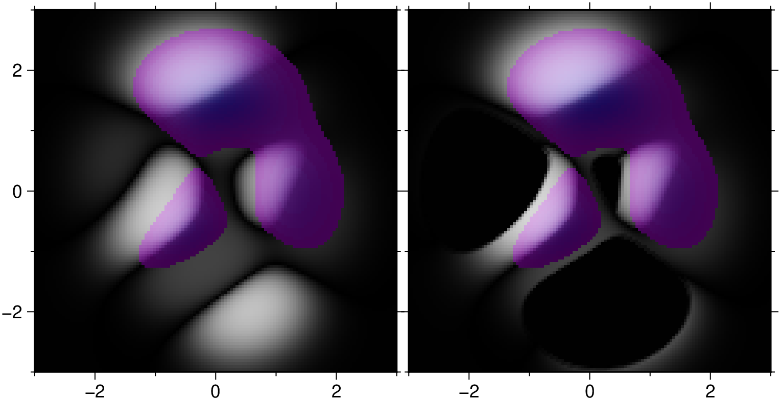
Fill the depressions of the peaks surface. Show original and sinks filled side by side.

using GMT

G = peaks(N=128);
G2 = fillsinks(G);
grdimage(G, figsize=6, shade=true)
grdimage!(G2, figsize=6, xshift=6.2, frame="wSen", shade=true, show=true)

Now save the filling contours n the SACO global variable and make a plot that overlayes them

using GMT

G = peaks(N=128);
G2 = fillsinks(G, saco=true);
grdimage(G2, shade=true)
plot!(get(GMT.SACO[1], "saco", nothing), lc=:white, show=true)

See Also