Arrow examples
arrows(cmd0::String="", arg1=nothing; arrow=(...), kwargs...)Plot an arrow field.
When the keyword arrow=(...) or vector=(...) is used, the direction (in degrees counter-clockwise from horizontal) and length must be found in columns 3 and 4, and size, if not specified on the command-line, should be present in column 5. The size is the length of the vector head. Vector stem width is set by option pen or line_attrib.
The vecmap=(...) variation is similar to above except azimuth (in degrees east of north) should be given instead of direction. The azimuth will be mapped into an angle based on the chosen map projection. If length is not in plot units but in arbitrary user units (e.g., a rate in mm/yr) then you can use the input_col option to scale the corresponding column via the +sscale modifier.
The geovec=(...) or geovector=(...) keywords plot geovectors. In geovectors, azimuth (in degrees east from north) and geographical length must be found in columns 3 and 4. The size is the length of the vector head. Vector width is set by pen or line_attrib. Note: Geovector stems are drawn as thin filled polygons and hence pen attributes like dashed and dotted are not available. For allowable geographical units, see the units=() option.
The full arrow options list can be consulted at Vector Attributes
B | frame | axis | xaxis yaxis:: [Type => Str]
Set map boundary frame and axes attributes.
J | proj | projection :: [Type => String]
Select map projection. Defaults to 15x10 cm with linear (non-projected) maps.
R | region | limits :: [Type => Str or list or GMTgrid|image] $Arg = (xmin,xmax,ymin,ymax)$
Specify the region of interest. Set to data minimum BoundinBox if not provided.
W | pen | line_attrib :: [Type => Str]
Set pen attributes for lines or the outline of symbols
savefig | figname | name :: [Type => Str]
Save the figure with the
figname=name.extwhereextchooses the figure format (e.g. figname="name.png")
Example:
arrows([0 8.2 0 6], limits=(-2,4,0,9), arrow=(len=2,stop=1,shape=0.5,fill=:red), axis=:a, pen="6p", show=true)using GMT
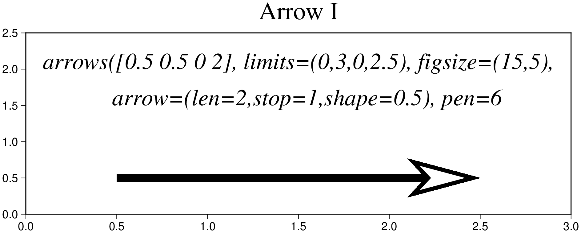
arrows([0.5 0.5 0 2], limits=(0.,3,0,2.5), figsize=(15,5),
arrow=(len=2,), pen=6,
frame=(axes=:WSrt, annot=:auto, title="Arrow I"))
# Add the plotting command to the figure
T1 = "arrows([0.5 0.5 0 2], limits=(0,3,0,2.5), figsize=(15,5),";
T2 = " arrow=(len=2,stop=1,shape=0.5), pen=6";
pstext!([1.5 2.0], text=T1, font=(18,"Times-Italic"), justify=:CB)
pstext!([1.5 1.5], text=T2, font=(18,"Times-Italic"), justify=:CB, show=true)
using GMT
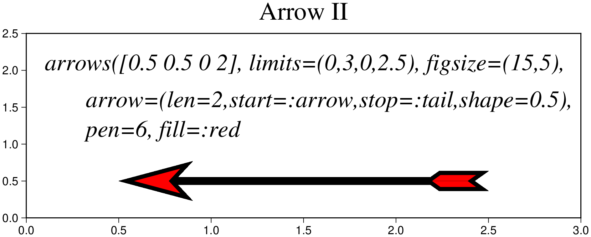
arrows([0.5 0.5 0 2], limits=(0,3,0,2.5), figsize=(15,5),
arrow=(len=2,start=:arrow,stop=:tail,shape=0.5), fill=:red, pen=6,
frame=(axes=:WSrt, annot=:auto, title="Arrow II"))
# Add the plotting command to the figure
T1 = "arrows([0.5 0.5 0 2], limits=(0,3,0,2.5), figsize=(15,5),";
T2 = " arrow=(len=2,start=:arrow,stop=:tail,shape=0.5),";
T3 = " pen=6, fill=:red";
pstext!([0.1 2.0], text=T1, font=(18,"Times-Italic"), justify=:LB)
pstext!([0.1 1.5], text=T2, font=(18,"Times-Italic"), justify=:LB)
pstext!([0.1 1.1], text=T3, font=(18,"Times-Italic"), justify=:LB, show=true)
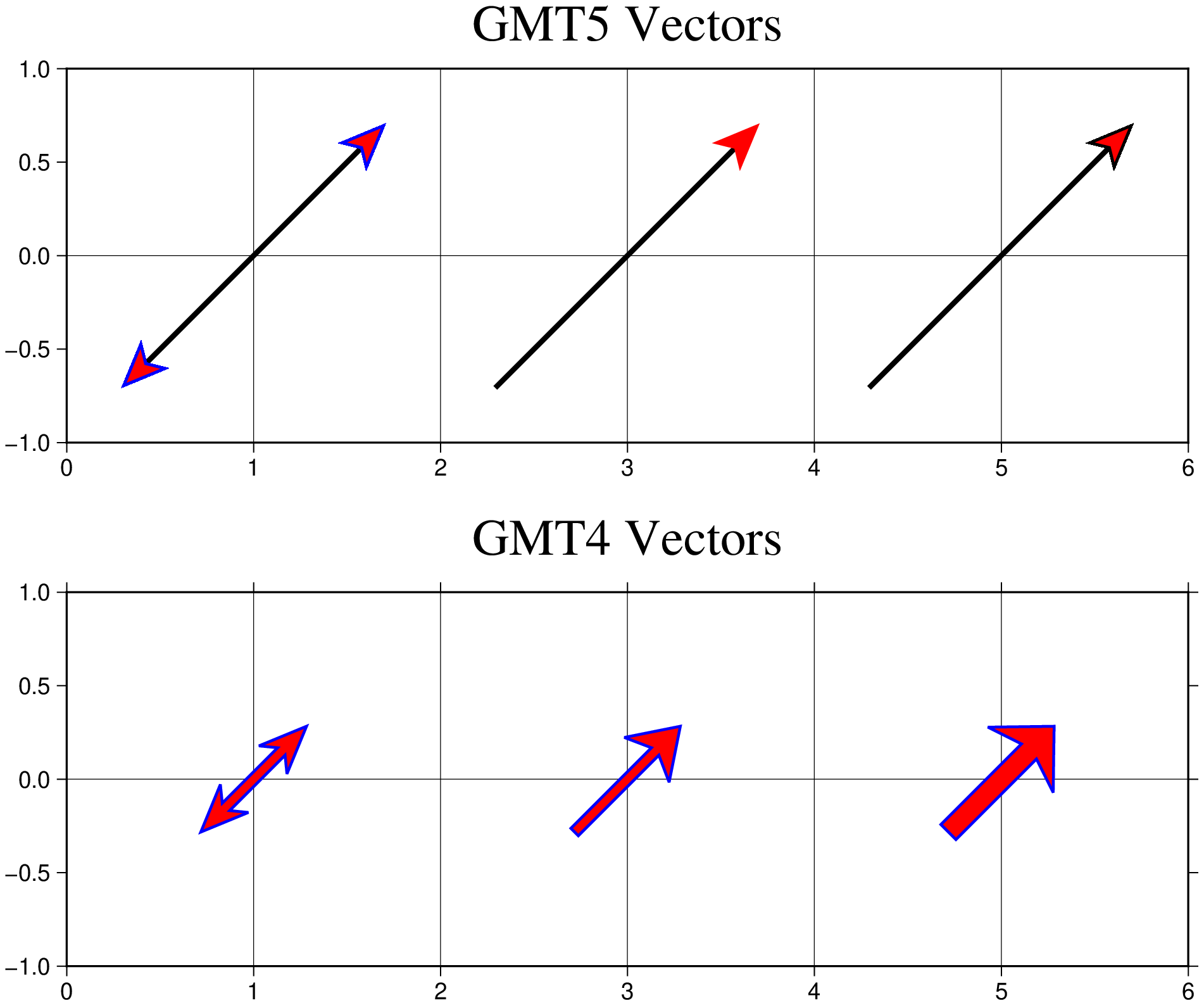
GMT4 & GMT5 style arrows
Plot GMT4 style arrows. We show here three alternatives to set arrow heads
using GMT
arrows([1 0 45 2], region=(0,6,-1,1), figscale="2.5",
       frame=(annot=:auto, grid=1, title="GMT4 Vectors"),
       pen=(1,:blue), fill=:red, arrow4=(align=:middle,
       head=(arrowwidth="4p", headlength="18p", headwidth="7.5p"), double=true))
arrows!([3 0 45 2], pen=(1,:blue), fill=:red,
        arrow4=(align=:middle, head=("4p","18p", "12p")))
arrows!([5 0 45 2], pen=(1,:blue), fill=:red,
        arrow4=(align=:middle, head="8p/18p/17.5p"))

# Now the GMT5 type arrows
arrows!([1 0 45 2], frame=(annot=:auto, grid=1, title="GMT5 Vectors"), lw=2, fill=:red,
        arrow=(length="18p", start=true, stop=true, pen=(1,:blue),
               angle=45, justify=:center, shape=0.5), yshift=7)
arrows!([3 0 45 2], lw=2, fill=:red,
        arrow=(length="18p", stop=true, pen="-", angle=45, justify=:center, shape=0.5))
arrows!([5 0 45 2], lw=2, fill=:red,
        arrow=(length="18p", stop=true, angle=45, justify=:center, shape=0.5), show=true)
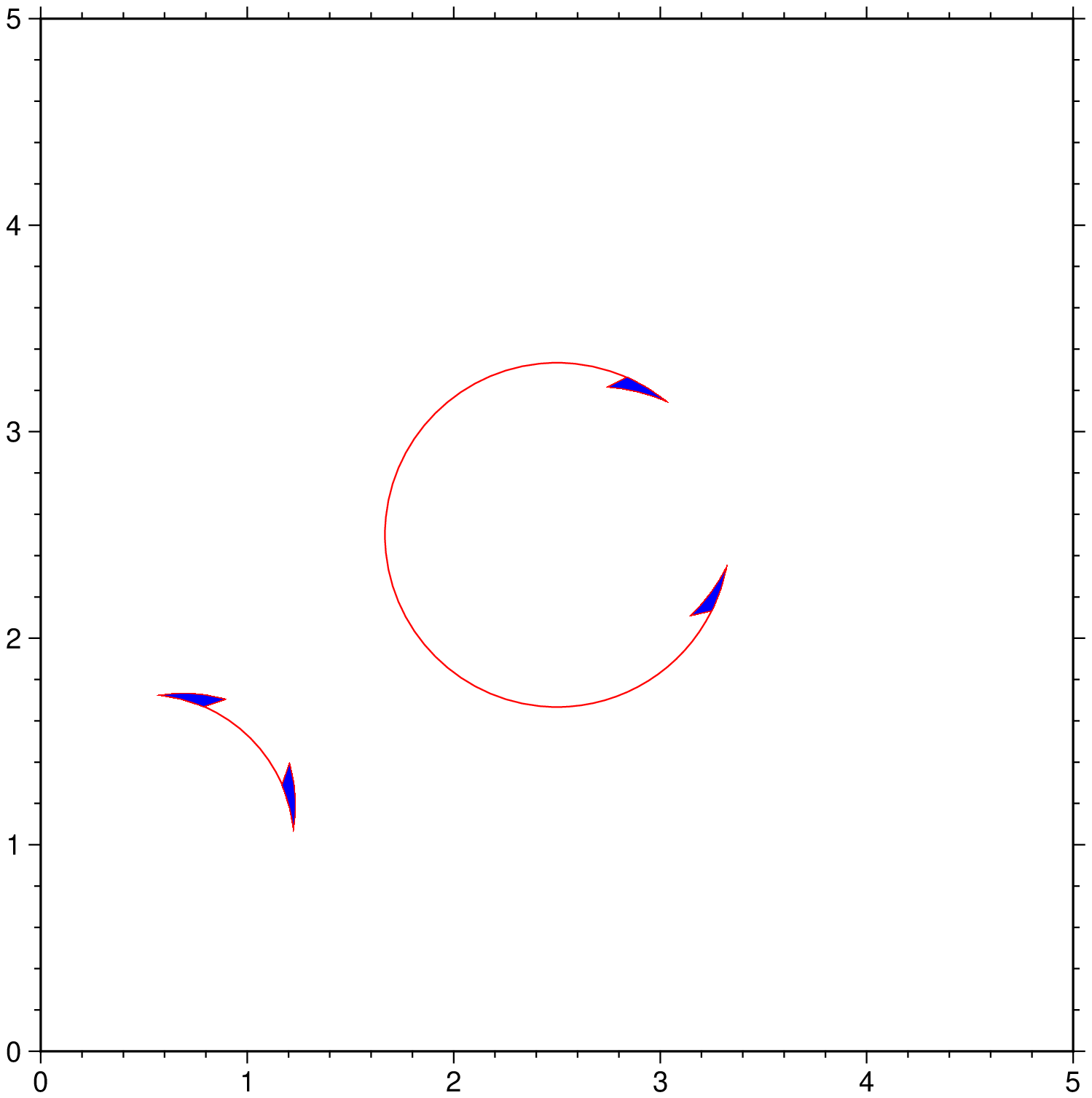
Mat angles
Plot matangle symbols with vector heads.
using GMT
plot([0.5 1 1.75 5 85], region=(0,5,0,5), figsize=12,
        marker=(matang=true, arrow=(length=0.75, start=true, stop=true, half=:right)),
        ml=(0.5,:red), fill=:blue)
# Now add another matangle symbol but transmit the angle parameters via the
# keyword. Note that in this case the arrow attributes are wrapped in a NamedTuple
plot!([2.5 2.5], marker=(:matang, [2 50 350], (length=0.75, start=true, stop=true, half=:left)),
        ml=(0.5,:red), fill=:blue, show=true)
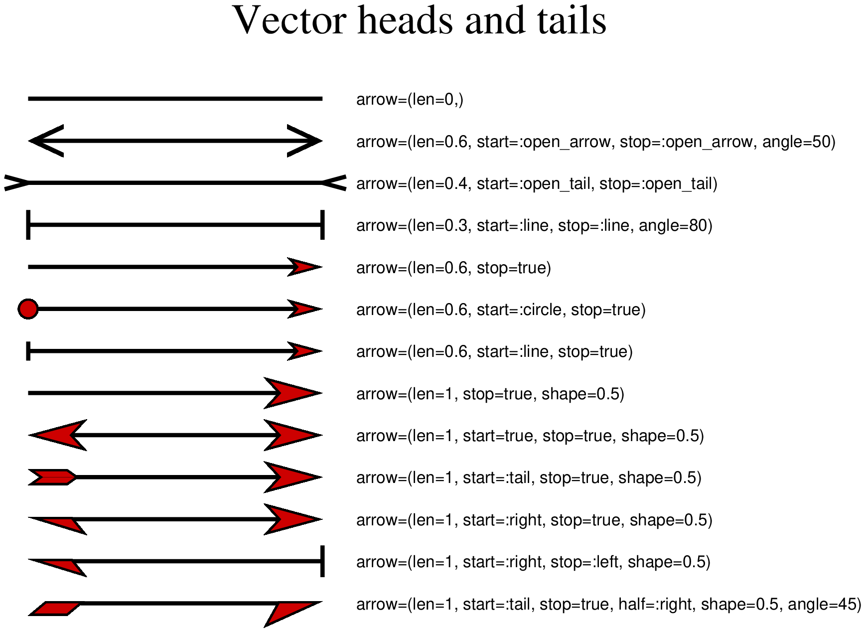
Vector heads and tails
There are many methods to plot vectors with individual heads and tails. For this purpose, several modifiers may be set to the corresponding vector-producing parameters for specifying the placement of vector heads and tails, their shapes, and the justification of the vector, see more at Vector Attributes.
using GMT

arrows([1 14 0 35], limits=(-5,100,1,15), figsize=(15,10), pen=2, arrow=(len=0,),
       frame=:none, title="Vector heads and tails")
text!(["arrow=(len=0,)"], x=40, y=14, font=8, justify=:LM)
arrows!([1 13 0 35], pen=2, arrow=(len=0.6, start=:open_arrow, stop=:open_arrow, angle=50))
text!(["arrow=(len=0.6, start=:open_arrow, stop=:open_arrow, angle=50)"], x=40, y=13, font=8, justify=:LM)
arrows!([1 12 0 35], pen=2, arrow=(len=0.4, start=:open_tail, stop=:open_tail))
text!(["arrow=(len=0.4, start=:open_tail, stop=:open_tail)"], x=40, y=12, font=8, justify=:LM)
arrows!([1 11 0 35], pen=2, arrow=(len=0.3, start=:line, stop=:line, angle=80))
text!(["arrow=(len=0.3, start=:line, stop=:line, angle=80)"], x=40, y=11, font=8, justify=:LM)
arrows!([1 10 0 35], pen=2, arrow=(len=0.6, stop=true), fill=:red3)
text!(["arrow=(len=0.6, stop=true)"], x=40, y=10, font=8, justify=:LM)
arrows!([1  9 0 35], pen=2, arrow=(len=0.6, start=:circle, stop=true), fill=:red3)
text!(["arrow=(len=0.6, start=:circle, stop=true)"], x=40, y=9, font=8, justify=:LM)
arrows!([1  8 0 35], pen=2, arrow=(len=0.6, start=:line, stop=true), fill=:red3)
text!(["arrow=(len=0.6, start=:line, stop=true)"], x=40, y=8, font=8, justify=:LM)
arrows!([1  7 0 35], pen=2, arrow=(len=1, stop=true, shape=0.5), fill=:red3)
text!(["arrow=(len=1, stop=true, shape=0.5)"], x=40, y=7, font=8, justify=:LM)
arrows!([1  6 0 35], pen=2, arrow=(len=1, start=true, stop=true, shape=0.5), fill=:red3)
text!(["arrow=(len=1, start=true, stop=true, shape=0.5)"], x=40, y=6, font=8, justify=:LM)
arrows!([1  5 0 35], pen=2, arrow=(len=1, start=:tail, stop=true, shape=0.5), fill=:red3)
text!(["arrow=(len=1, start=:tail, stop=true, shape=0.5)"], x=40, y=5, font=8, justify=:LM)
arrows!([1  4 0 35], pen=2, arrow=(len=1, start=:right, stop=true, shape=0.5), fill=:red3)
text!(["arrow=(len=1, start=:right, stop=true, shape=0.5)"], x=40, y=4, font=8, justify=:LM)
arrows!([1  3 0 35], pen=2, arrow=(len=1, start=:right, stop=:left, shape=0.5), fill=:red3)
text!(["arrow=(len=1, start=:right, stop=:left, shape=0.5)"], x=40, y=3, font=8, justify=:LM)
arrows!([1  2 0 35], pen=2, arrow=(len=1, start=:tail, stop=true, half=:right, shape=0.5, angle=45), fill=:red3)
text!(["arrow=(len=1, start=:tail, stop=true, half=:right, shape=0.5, angle=45)"], x=40, y=2, font=8, justify=:LM)
showfig()
Cartesian, circular, and geographic vectors
Plot Cartesian, circular, and geographic vectors. This example was picked from the PyGMT gallery.
using GMT
coast(region=[-127, -64, 24, 53], proj=:merc, borders=1, area=4000, shore=true)

# Left: plot 12 Cartesian vectors with different lengths
x = fill(-117, 12);               # x vector coordinates
y = linspace(33.5, 42.5, 12);     # y vector coordinates
direction = zeros(12);            # direction of vectors (horizontal)
length = linspace(2, 10, 12);  # length of vectors
arrows!([x y direction length], pen=(1,:red),
        arrow=(len="0.2", stop=true, fill=:red, angle=40, shape=:triang))
text!(text="CARTESIAN", x=-112, y=44.2, font="13p,Helvetica-Bold,red")

# Middle: plot 7 math angle arcs with different radii
num = 7
x, y = fill(-95, 7), fill(37, 7)
radius = 1.8 .- 0.2 * (0:num-1)
startdir = fill(90, num)
stopdir  = 180 .+ 40 * (0:num-1)
data = [x y radius startdir stopdir]
plot!(data, marker=(matang=true, arrow=(length=0.5, stop=true)), fill=:red3, pen="1.5,black")
text!(text="CIRCULAR", x=-95, y=44.2, font="13p,Helvetica-Bold,black")

# Right: plot geographic vectors using endpoints
NYC = [-74.0060 40.7128]
CHI = [-87.6298 41.8781]
SEA = [-122.3321 47.6062]
NO = [-90.0715 29.9511]
plot!([NYC CHI; NYC SEA; NYC NO], pen="1.0,blue",
      geovec=(length=0.5, stop=true, endpoint=true, fill=:blue, angle=30, pen="1p,blue"))
text!(text="GEOGRAPHIC", x=-74.5, y=44.2, font="13p,Helvetica-Bold,blue", show=1)

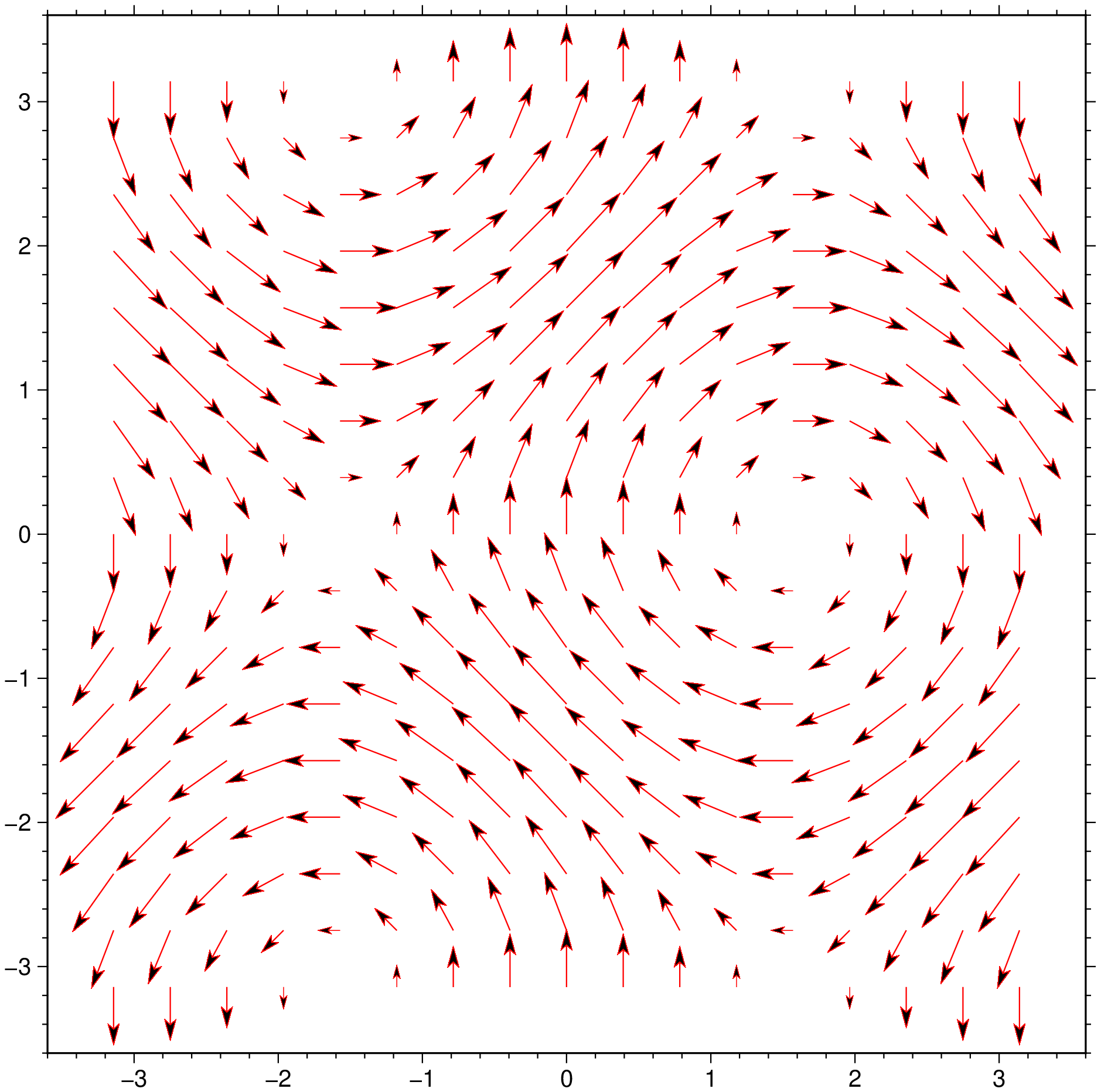
Quivers
A (nicer looking) Matlab quiver plot example. To fully reproduce the Matlab example we also use the extremely memory wasting meshgrid. And because we turn U and V into grids before sending them to GMT, not specifying the limits would lose all first/last column/rows because most of the arrows are going out of the grid domain. We could have done it but it looks nicer if we specify a slightly wider domain.
using GMT
X,Y = meshgrid(-pi:pi/8:pi,-pi:pi/8:pi);
U = sin.(Y);
V = cos.(X);
quiver(X, Y, U, V, region=(-3.6,3.6,-3.6,3.6), fill=:black, lc=:red, show=true)
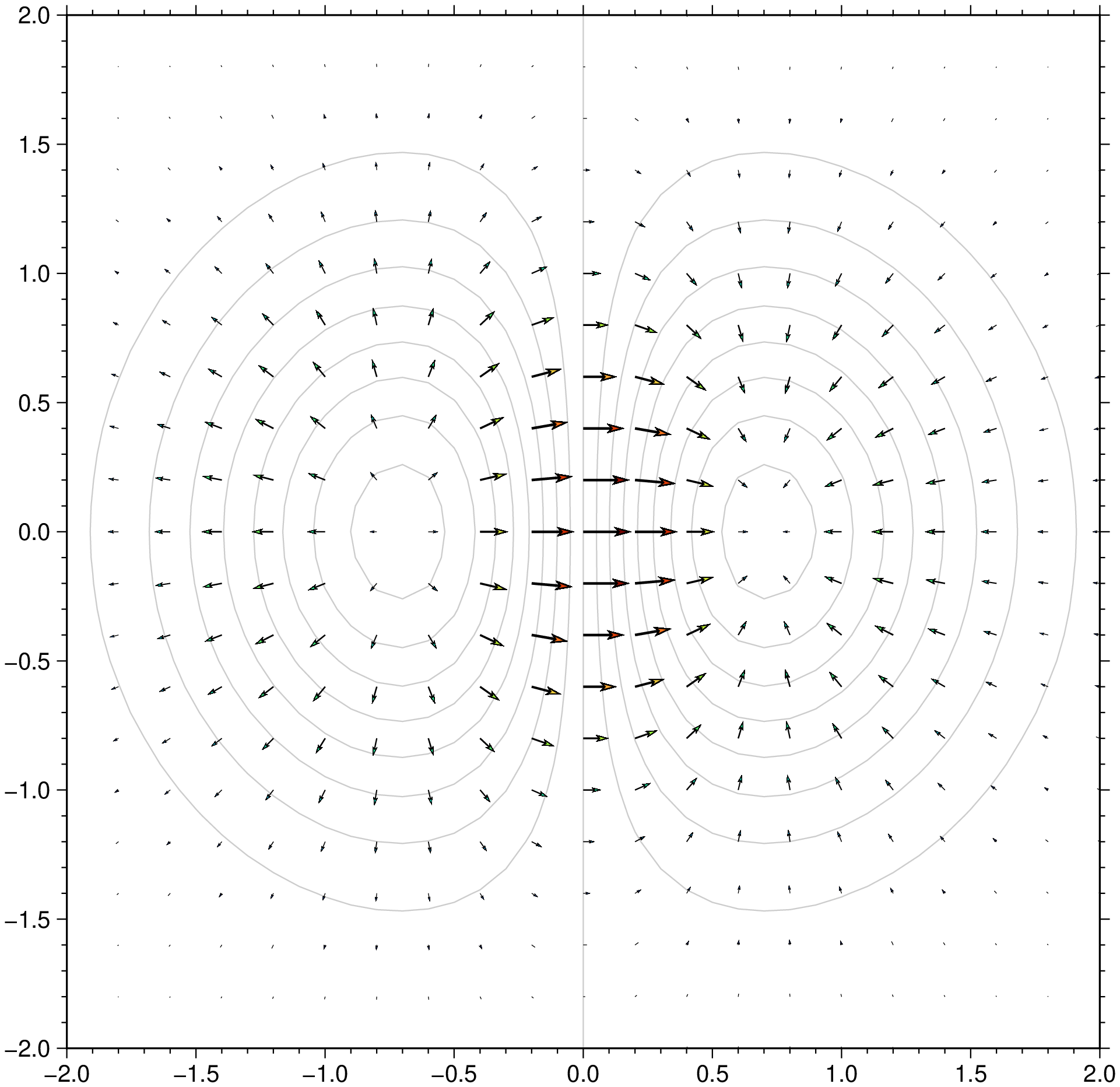
Next example doesn't need our help to extend the plotting limits and it uses grids directly. And for simplicity let's create a grid using grdmath and compute its horizontal derivatives. Then we plot them as an arrow field.
using GMT
G = gmt("grdmath -R-2/2/-2/2 -I0.1 X Y R2 NEG EXP X MUL");
dzdy = gmt("grdmath ? DDY", G);
dzdx = gmt("grdmath ? DDX", G);
grdcontour(G, annot=:none, pen=:gray80)
grdvector!(dzdx, dzdy, cmap=:turbo, lw=1, show=true)
The above examples used Cartesian coordinates, but we can use also geographic coordinates where the arrows know where they are on Earth. This example plots the NUVEL1 plate motion model velocities relative to the Eurasian plate. The defaults guess pretty much a good solution for the arrow's length and header sizes, but we can modify them if we are not satisfied with the default results.
using GMT
quiver(TESTSDIR * "assets/nuvel1_vx.nc", TESTSDIR * "assets/nuvel1_vy.nc", proj=:guess,
       coast=(shore=:gray70, area=5000), lw=1, C=:turbo, show=true, Vd=1)
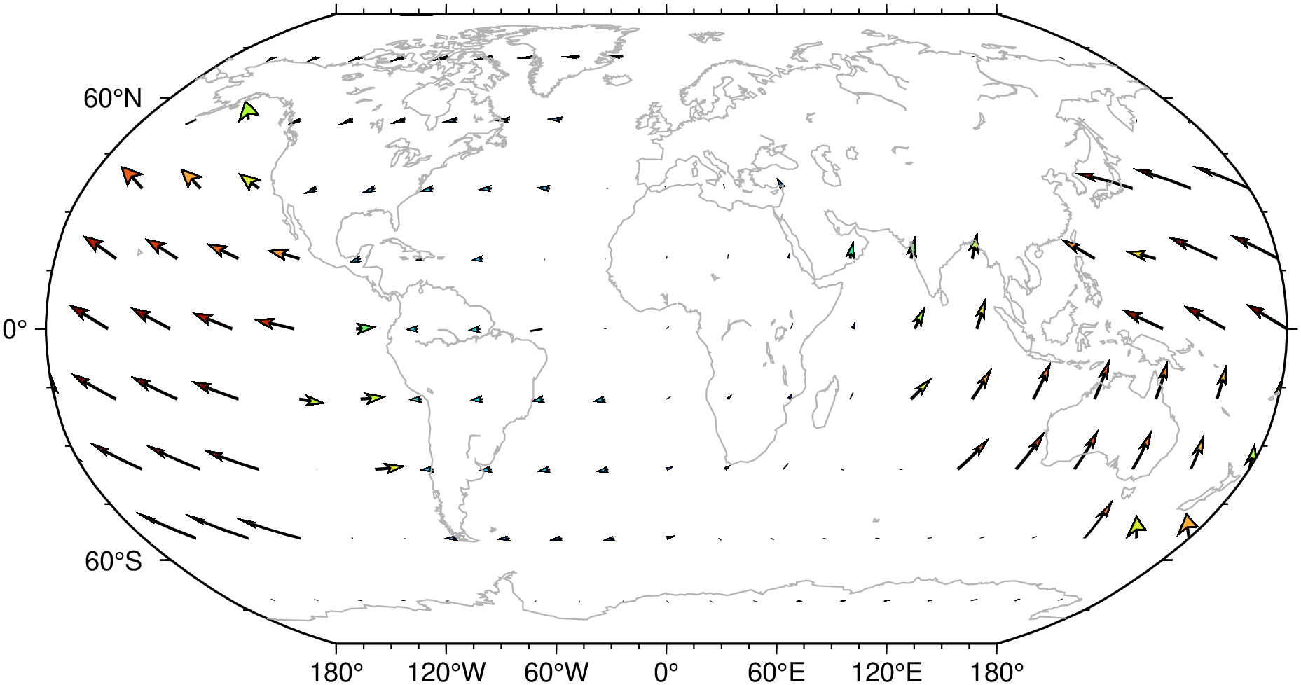
A nice and instructive plot but we may want a somewhat larger arrows. Figuring out a best sized arrows is very tricky and no solution will please all users. The above command used the option Vd=1, which prints the real hard core command that is sent to GMT. Many users get scared with it but fine tuning implies understanding its contents. Specifically the -Si136.92637k part that sets arrows scale factor. Much more information is provided in the grdvector manual page, but as a quick help here we inform that i stands for inverse scale factor (136.92637 in this case) and k means kilometers. So if we want larger arrows we must increase the (inverse) scale factor. A slightly modified version of the above is obtained with:
using GMT
quiver(TESTSDIR * "assets/nuvel1_vx.nc", TESTSDIR * "assets/nuvel1_vy.nc", proj=:guess, lw=1,
       coast=(shore=:gray70, area=5000), vscale=(inverse=true, scale="400k"), C=:turbo, show=true)
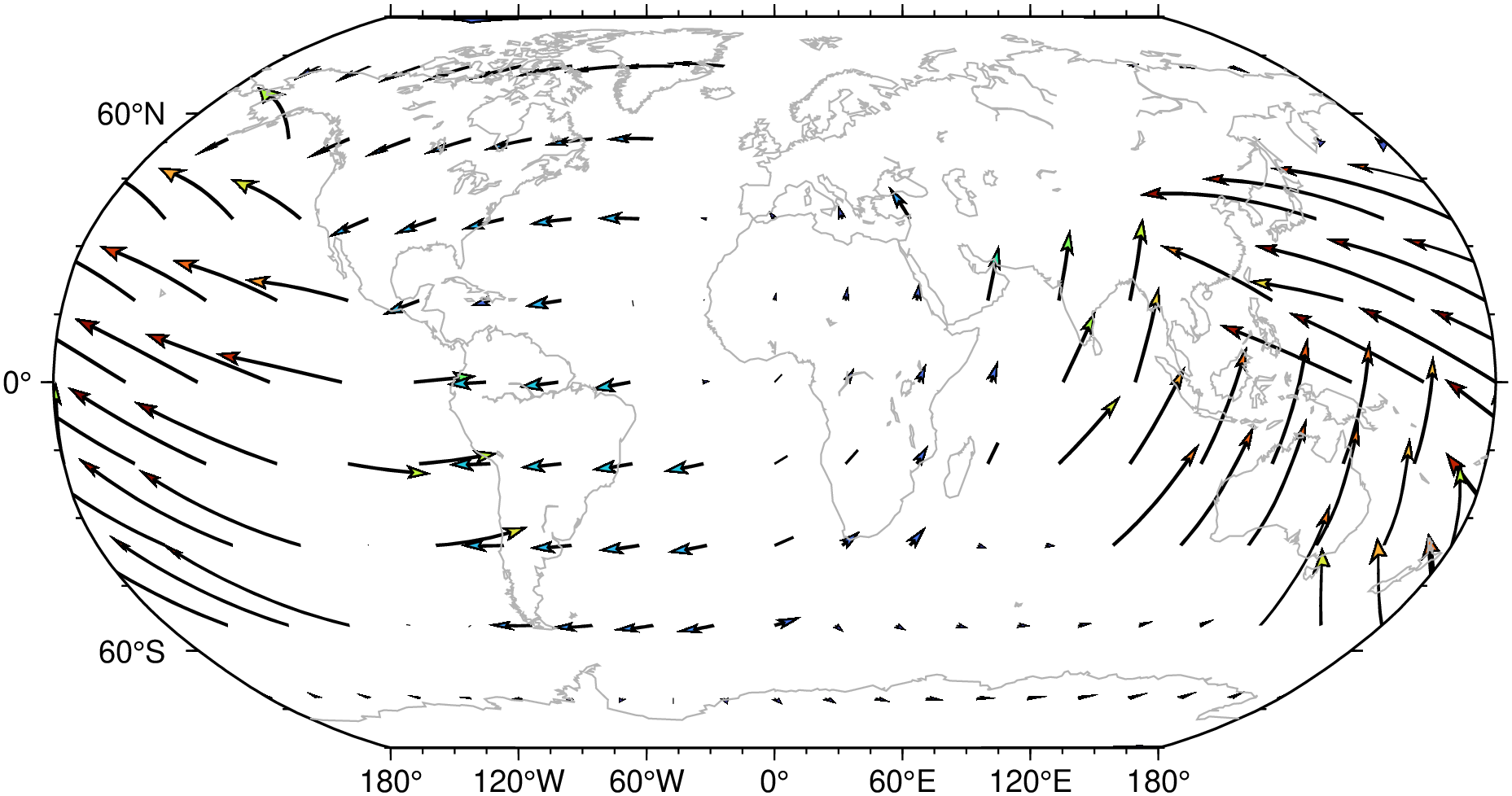
Here we exaggerated on the arrow scale to show the other side of the problem. If arrows are too long chances are high that they intersect.
These docs were autogenerated using GMT: v1.33.1