Line plots
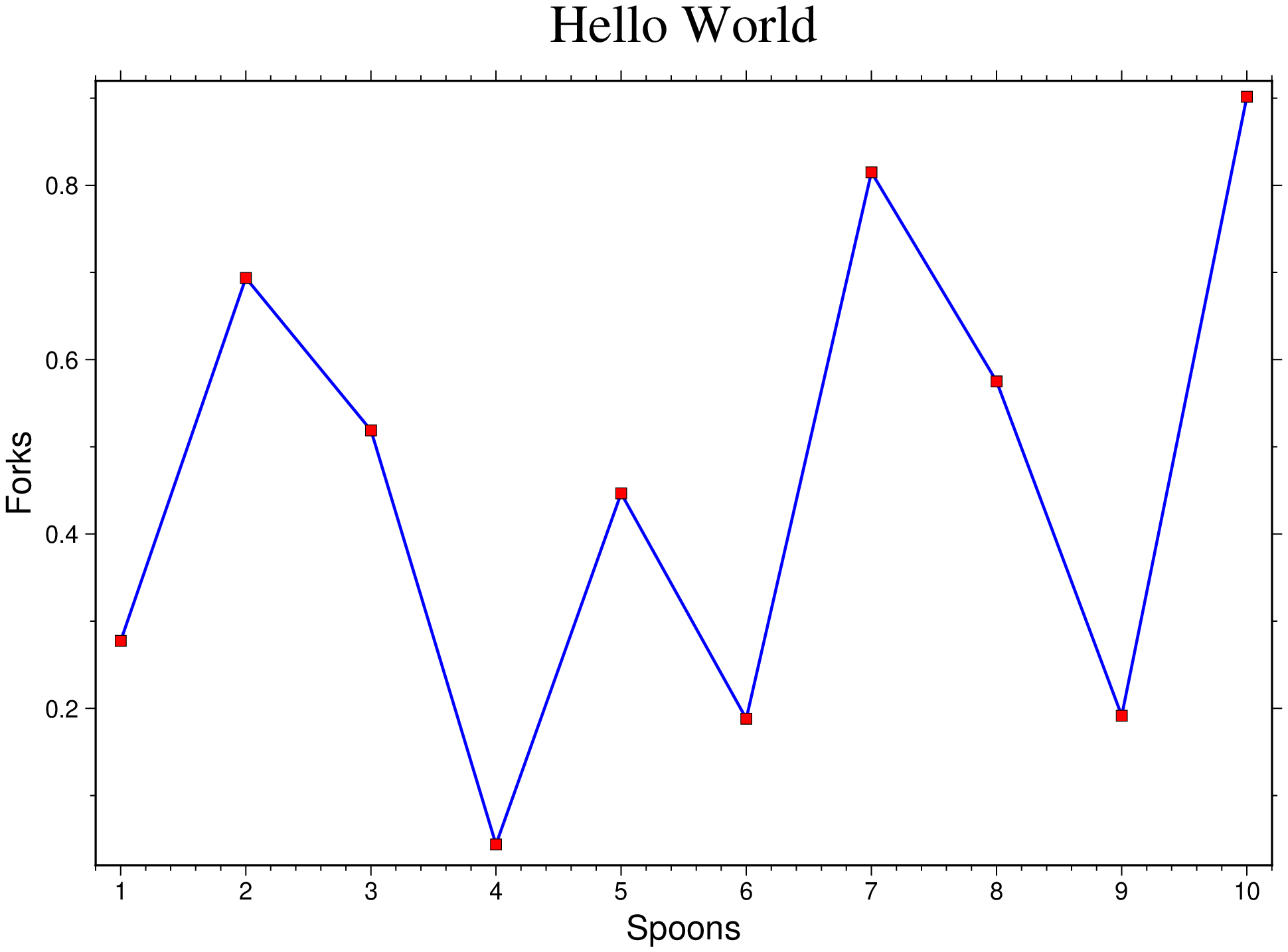
Hello world
using GMT
plot(1:10, rand(10), lw=1, lc=:blue, marker=:square,
     markeredgecolor=0, size=0.2, markerfacecolor=:red, title="Hello World",
     xlabel="Spoons", ylabel="Forks", show=true)
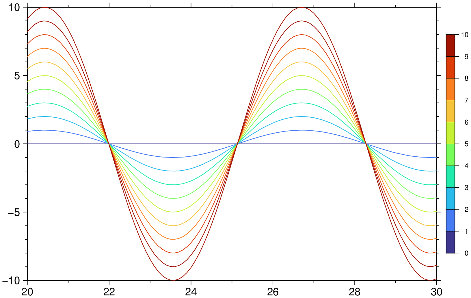
In this example the lines color is set using a custom CPT. Pen thickness is assigned automatically.
The custom CPT is used by setting the plot command’s cmap argument to true. This workas because we previously computed the CPT and it will remain in memory until it's consumed when we finish the plot. The level argument sets the color to be used from the custom CPT.
In fact, in this case with a CPT already in memory, the level option alone would have triggered the line coloring and the cmap option could have been droped.
Normally we don't need to start a figure with a call to basemap because the plot function takes care of guessing reasonable defaults, but in this case we start with a curve with small amplitude and we grow the figure by adding more lines. So if we leave it to automatic guessing one would have to start by the largest amplitude curve.
using GMT
C = makecpt(range=(0,10,1));
basemap(region=(20,30,-10,10), figsize=(12,8))
x = 20:0.1:30;
for amp = 0:10
	yy = amp .* sin.(x)
	plot!(x, yy, cmap=true, level=(data=amp, nofill=true))
end
colorbar!(show=true)
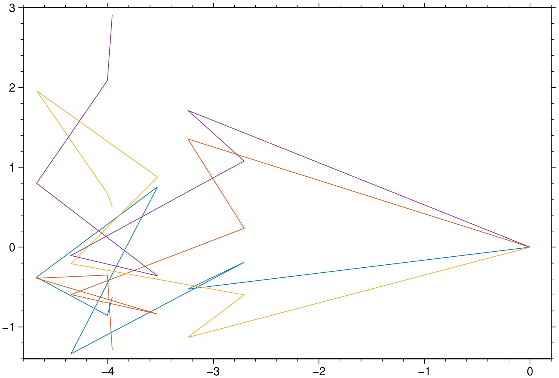
Line colors with the automatic color scheme
Here we are showing how to plot several lines at once and color them according to a circular color scheme comprised of 7 distinct colors. We start by generating a dummy matrix 8x5, where rows represent the vertex and the columns hold the lines. To tell the program that first column contains the coordinates and the remaining are all lines to be plotted we use the option multicol=true
using GMT
mat = GMT.fakedata(8, 5);
lines(mat, multicol=true, show=true)
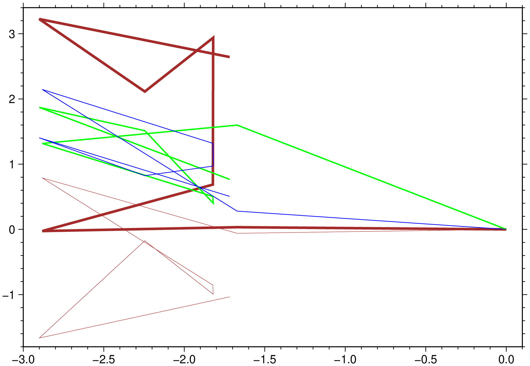
Line colors with user set color scheme
But if we want choose the colors ourselves, it is also easy though we need to go a bit lower in the data preparation.
The basic data type to transfer tabular data to GMT is the GMTdataset and the above command has converted the matrix into a GMTdataset under the hood but now we need to create one ourselves and fine control more details, like the colors and line thickness of the individual lines. Not that we have 5 lines but will provide 3 colors and 3 lines thicknesses. When we do this those properties are wrapped modulo its number.
using GMT
mat = GMT.fakedata(8, 5);
D = mat2ds(mat, color=["brown", "green", "blue"], linethick=[2, 1.0, 0.5, 0.25], multi=true);

# And now we just call *lines* (but using *plot* would have been the same) with the **D** argument.

lines(D, figsize=(14, 9.5), show=true)
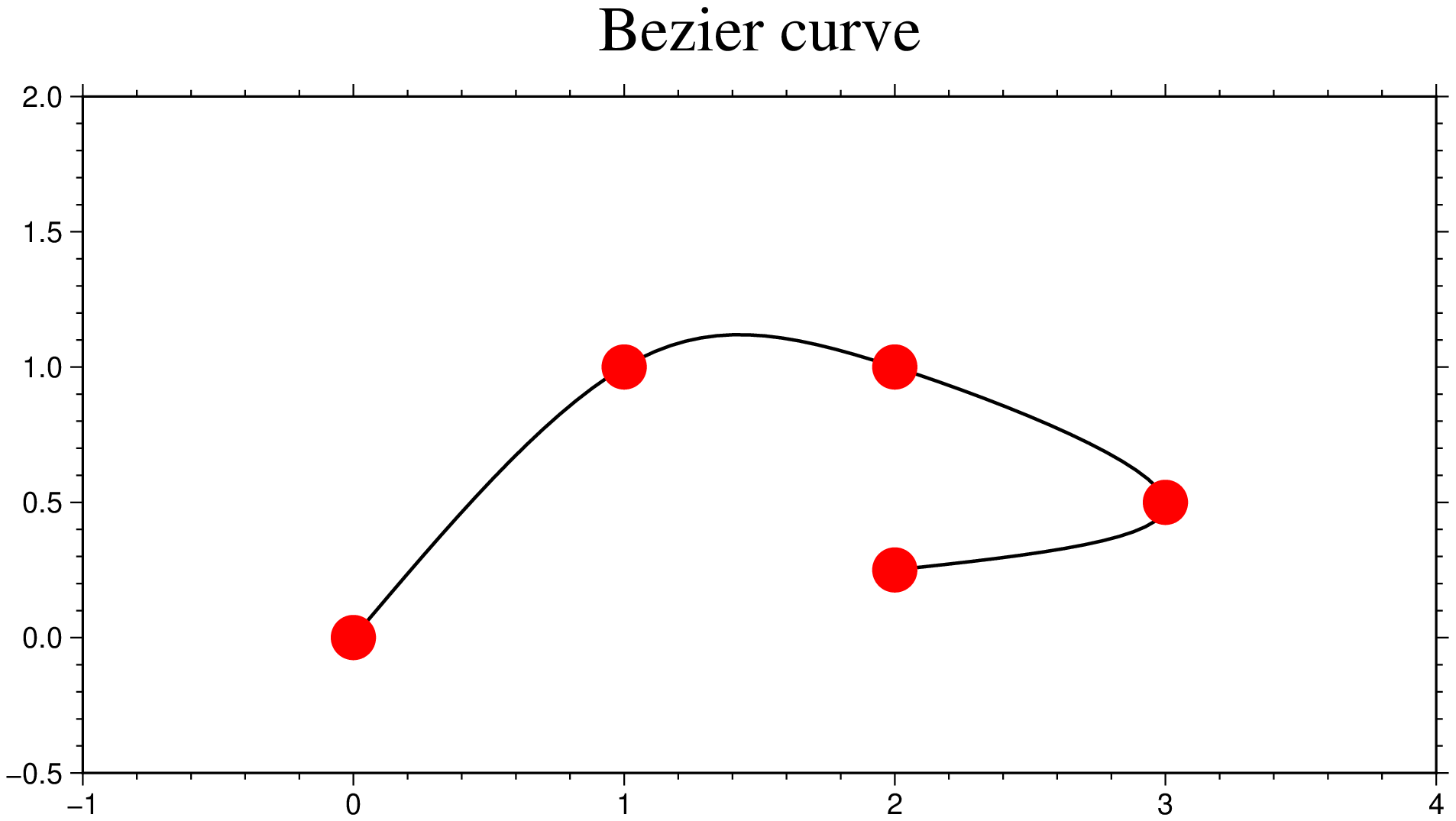
Bezier curve
using GMT
x = [0, 1, 2, 3, 2];  y = [0, 1, 1, 0.5, 0.25];
lines(x,y, limits=(-1,4,-0.5,2.0), scale=3.0, lw=1, markerfacecolor=:red,
      size=0.5, bezier=true, title="Bezier curve", show=true)
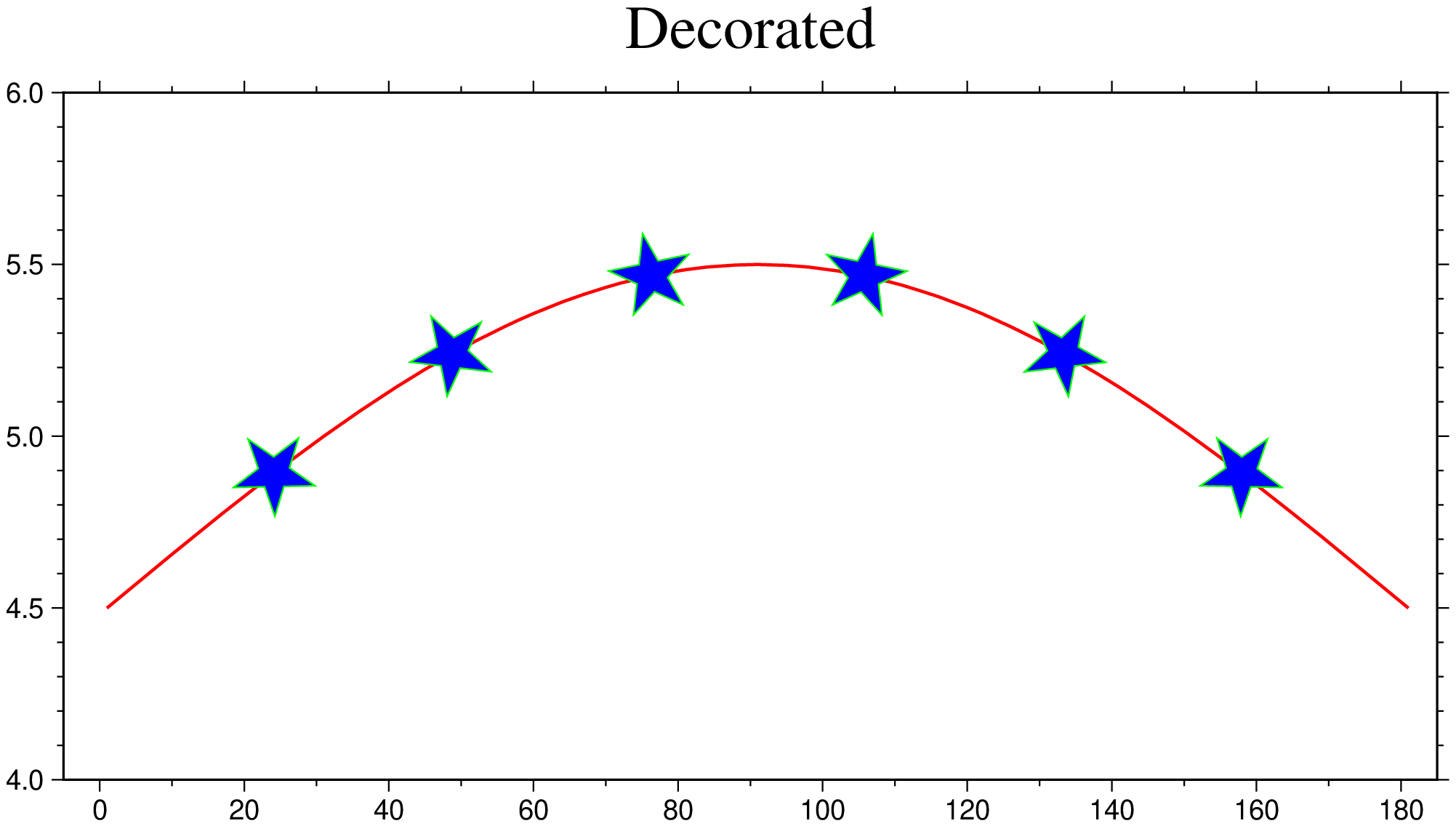
Decorated line
using GMT
xy = sind.(0:180) .+ 4.5
lines(xy, limits=(-5,185,4,6), figsize=(16,8), pen=(1,:red),
      decorated=(dist=(2.5,0.25), symbol=:star, size=1,
                 pen=(0.5,:green), fill=:blue, dec2=true),
      title=:Decorated, show=true)
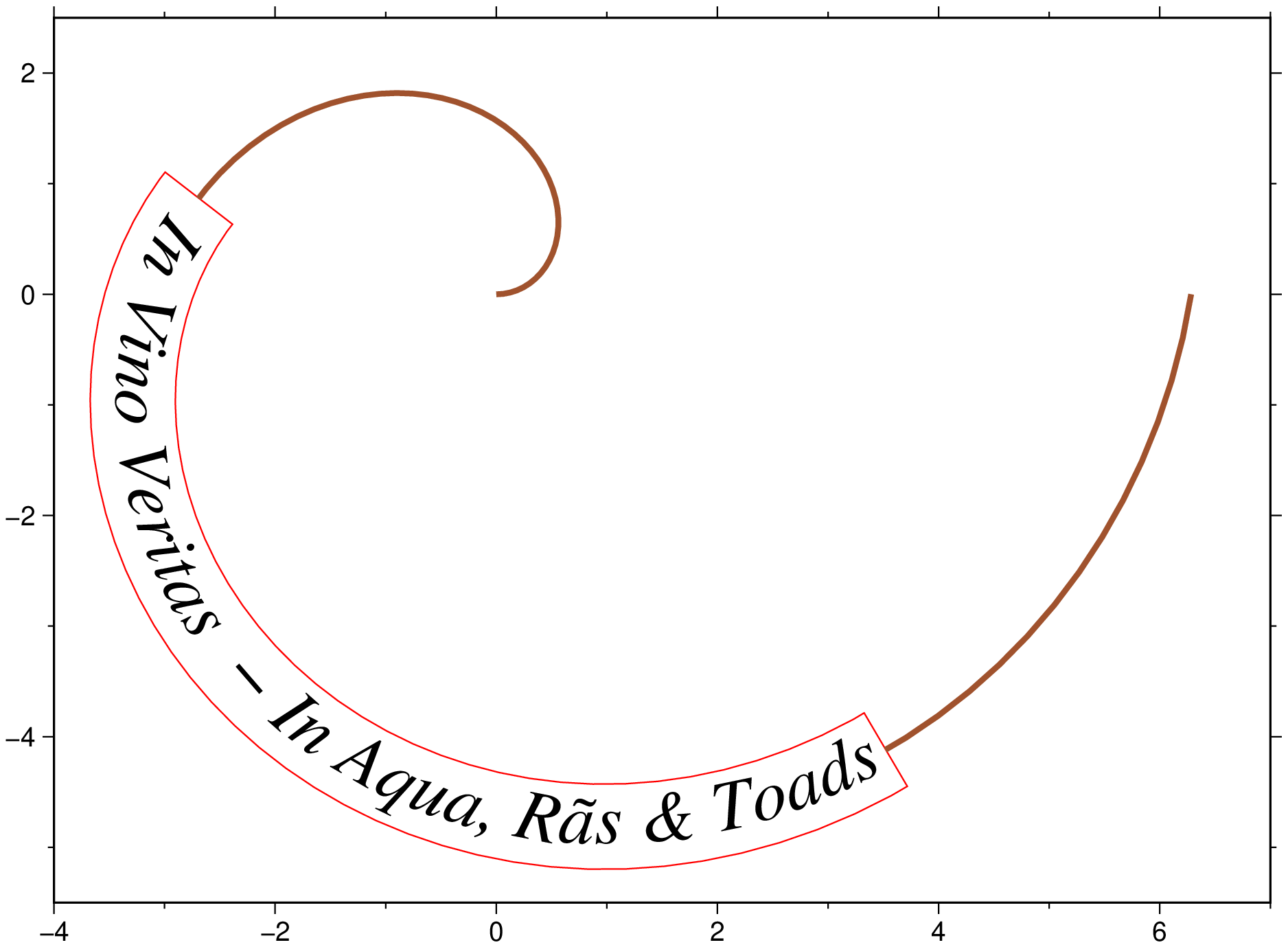
Text decorated line
using GMT
# Create a log spiral
t = linspace(0,2pi,100);
x = cos.(t) .* t;       y = sin.(t) .* t;
txt = " In Vino Veritas  - In Aqua, Rãs & Toads"
lines(x,y, region=(-4,7,-5.5,2.5), lw=2, lc=:sienna,
      decorated=(quoted=true, const_label=txt, font=(25,"Times-Italic"),
                 curved=true, pen=(0.5,:red)),
      aspect=:equal, show=true)
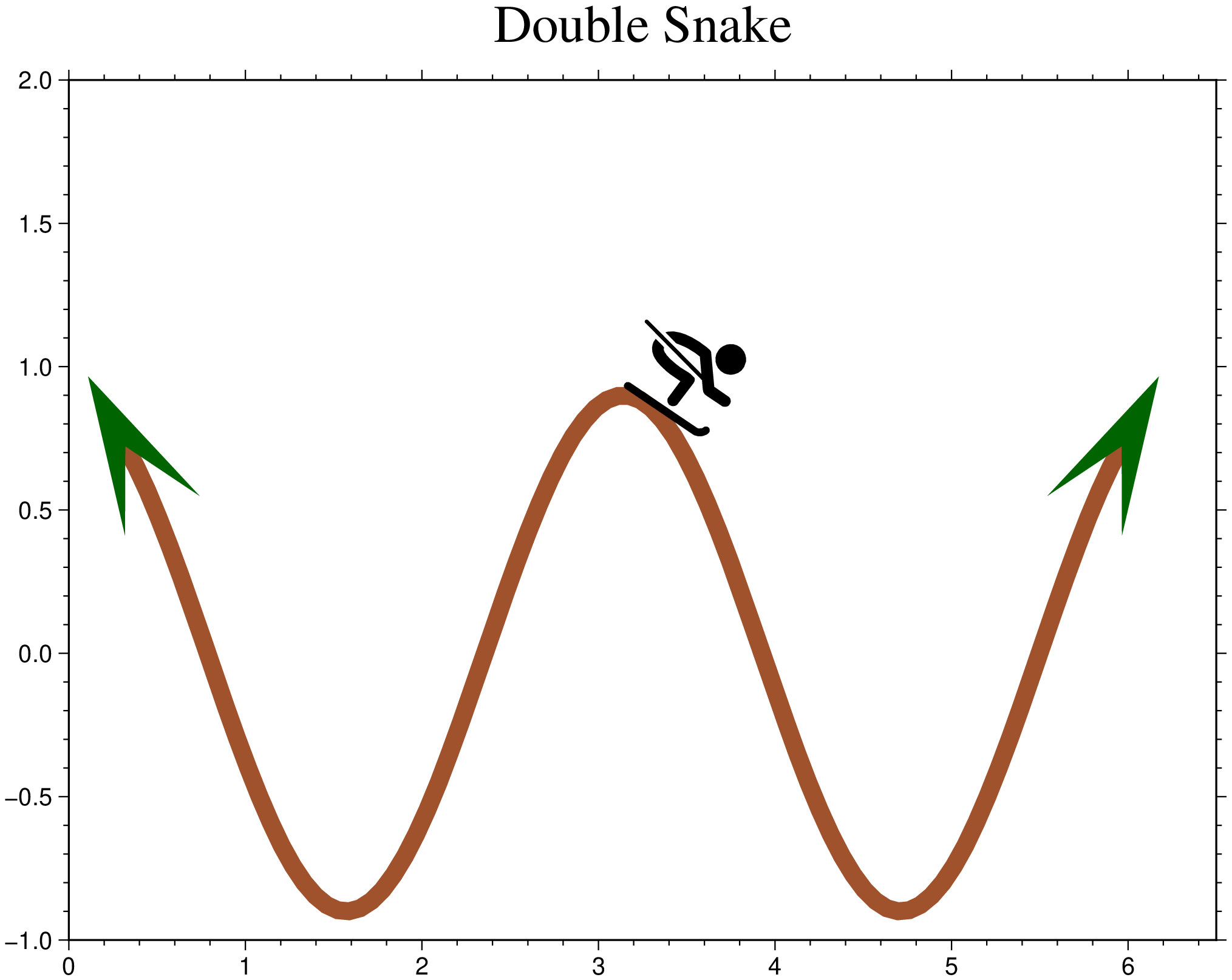
The snake skier
Plot a skier on a sinusoid.
using GMT

x = GMT.linspace(0, 2pi);  y = cos.(2x)*0.9;

lines(x,y,                           # The data
      limits=(0,6.5,-1,2.0),         # Fig limits
      pen=(lw=7,lc=:sienna, arrow=(len=2.2,shape=:arrow, fill=:darkgreen)),  # The "Snake"
      figsize=(16,12),               # Fig size
      title="Double Snake")
plot!(3.49, 0.97,                    # Coordinates where to plot symbol
      custom_symbol=(name="ski_alpine", size=1.7),    # The skier symbol
      fill=:black, show=true)        # Fill the symbol in black
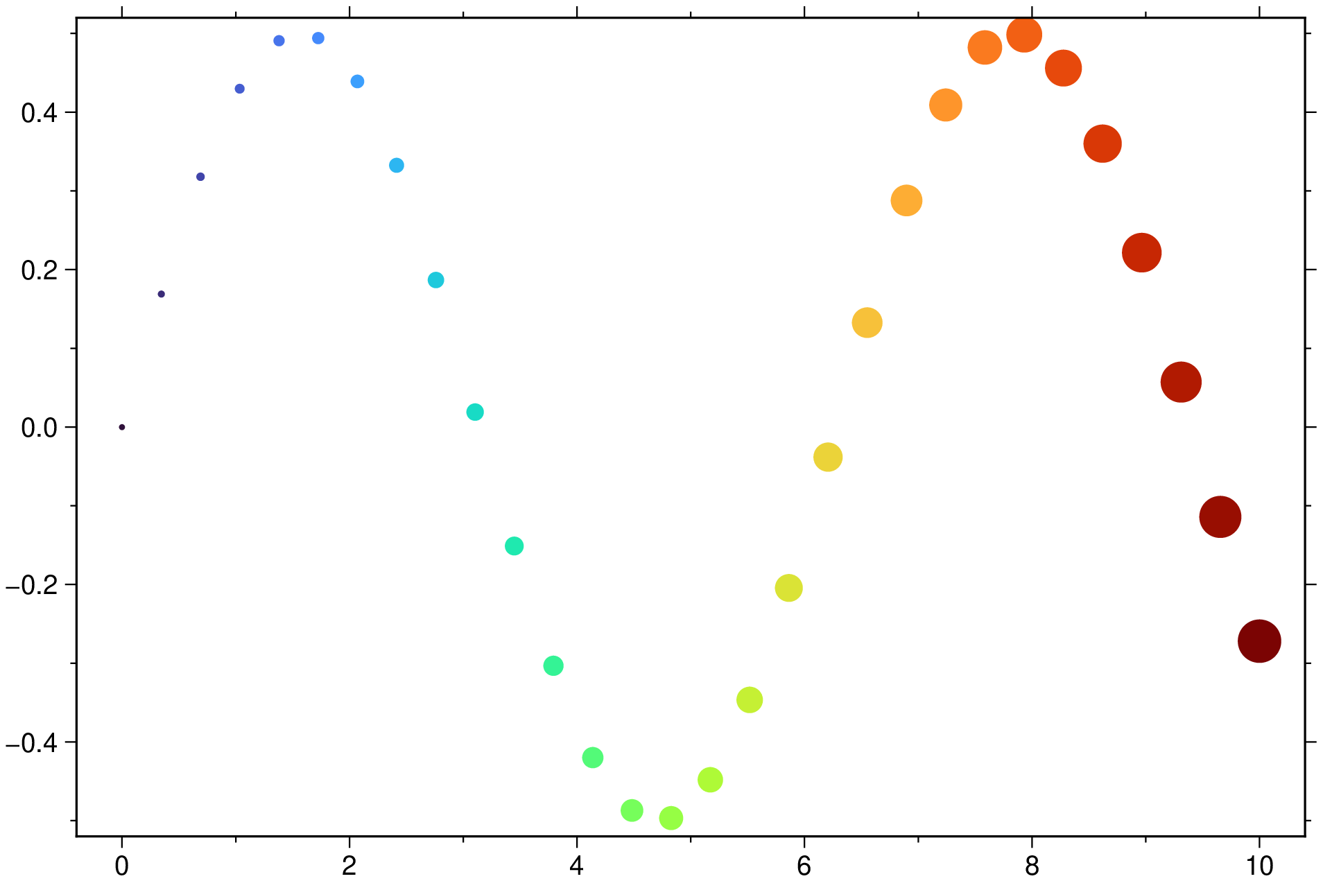
Variable sized/colors points
using GMT
xs = linspace(0,10,30);
ys = 0.5 .* sin.(xs);
scatter(xs, ys, zcolor=true, ms=linspace(2,15,30).*2.54/72, show=true)
These docs were autogenerated using GMT: v1.11.0