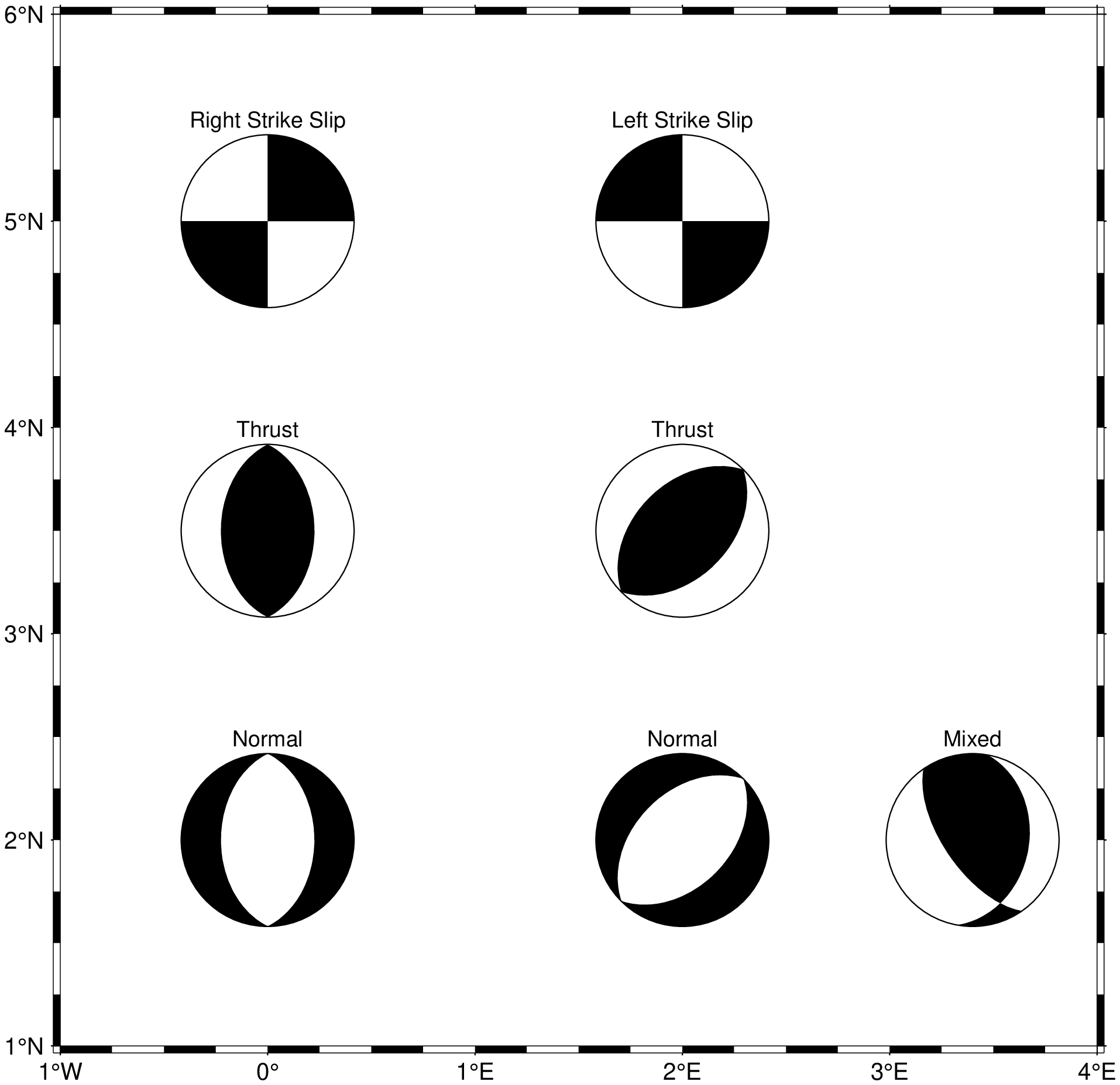
Focal mechanisms
Plotting beach balls (seismic focal mechanisms) in Julia using GMT.
Plotting beach balls
In this synthetic example we will use the Aki-Richards convention and pass the data via a GMTdataset
using GMT

# Right lateral Strike Slip
D = mat2ds([0.0 5.0 0.0 0 90 0 5 0 0],["Right Strike Slip"]);
meca(D, region=(-1,4,1,6), proj=:Mercator, aki=2.5, fill=:black)

# Left lateral Strike Slip
D = mat2ds([2.0 5.0 0.0 0 90 180 5 0 0],["Left Strike Slip"]);
meca!(D, aki=2.5, fill=:black)

# Thrust (two fault orientations)
D = mat2ds([0.0 3.5 0.0 0 45 90 5 0 0; 2.0 3.5 0.0 45 45 90 5 0 0],["Thrust", "Thrust"]);
meca!(D, aki=2.5, fill=:black)

# Normal (two fault orientations)
D = mat2ds([0.0 2.0 0.0 0 45 -90 5 0 0; 2.0 2.0 0.0 45 45 -90 5 0 0],["Normal", "Normal"]);
meca!(D, aki=2.5, fill=:black)

# Mixed
D = mat2ds([3.4 2.0 0.0 10 35 129 5 0 0],["Mixed"]);
meca!(D, aki=2.5, fill=:black)

showfig()
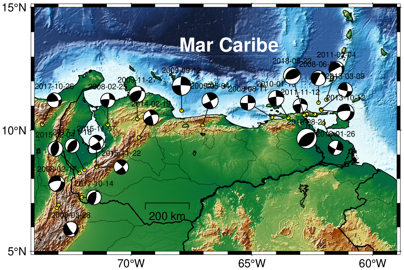
Some Venezuela beach balls
This example was presented by Leonardo Alvarado in the Showcase section of GMT forum under the title Map of focal mechanism with Pygmt. The example was slightly reworked and it now ues the GMT's automatic grid selection service that by using the grid name @earth_relief downloads the best resolution grid for the job.
The "mff_bb.txt" file contains a couple of focal mechanisms for the Venezuela region specified in the CMT convention format.
#D = gmtread(getpath4docs("mff_bb.txt"))
D = gmtread(GMT.TESTSDIR * "mff_bb.txt")| lon | lat | depth | str1 | dip1 | slip1 | str2 | dip2 | slip2 | mant | exp | plon | plat | Time |
|---|---|---|---|---|---|---|---|---|---|---|---|---|---|
| -73.069 | 6.801 | 161.7 | 19.0 | 51.0 | -143.5 | 264.0 | 62.4 | -45.2 | 5.5 | 0.0 | -73.069 | 7.801 | 1.20321e9 |
| -70.96 | 10.219 | 4.6 | 6.0 | 73.0 | 13.5 | 272.0 | 77.1 | 162.5 | 5.0 | 0.0 | -70.96 | 11.219 | 1.2039e9 |
| -72.989 | 6.912 | 160.9 | 41.0 | 37.0 | -16.1 | 144.0 | 80.4 | -125.9 | 5.2 | 0.0 | -72.489 | 5.912 | 1.20666e9 |
| -62.244 | 11.126 | 128.2 | 207.0 | 87.0 | -59.1 | 302.0 | 31.0 | -174.2 | 5.2 | 0.0 | -62.244 | 12.126 | 1.21452e9 |
| -64.168 | 10.523 | 13.7 | 90.0 | 86.0 | 0.0 | 360.0 | 90.0 | -4.0 | 5.2 | 0.0 | -65.168 | 11.123 | 1.21841e9 |
| -67.03 | 10.206 | 1.6 | 64.0 | 85.0 | 180.0 | 154.0 | 90.0 | 5.0 | 5.6 | 0.0 | -66.73 | 11.206 | 1.2414e9 |
| -67.909 | 10.807 | 5.8 | 270.0 | 83.0 | -171.8 | 179.0 | 81.9 | -7.1 | 6.4 | 0.0 | -67.909 | 11.807 | 1.25271e9 |
| -69.744 | 10.464 | 5.0 | 19.0 | 51.0 | 48.1 | 254.0 | 54.7 | 129.5 | 5.6 | 0.0 | -69.744 | 11.464 | 1.25928e9 |
| -63.494 | 10.505 | 5.0 | 267.0 | 74.0 | 180.0 | 357.0 | 90.0 | 16.0 | 5.4 | 0.0 | -63.994 | 11.305 | 1.26351e9 |
| -61.92 | 11.25 | 137.4 | 338.0 | 33.0 | -172.9 | 242.0 | 86.1 | -57.2 | 5.3 | 0.0 | -61.5 | 12.5 | 1.29678e9 |
| -62.4 | 10.65 | 62.3 | 268.0 | 69.0 | 171.7 | 1.0 | 82.2 | 21.2 | 5.0 | 0.0 | -63.0 | 11.0 | 1.32106e9 |
| -62.14 | 10.85 | 100.5 | 101.0 | 80.0 | 26.7 | 6.0 | 63.7 | 168.8 | 5.0 | 0.0 | -61.14 | 11.65 | 1.36279e9 |
| -62.12 | 10.82 | 67.9 | 15.0 | 45.0 | -155.3 | 267.0 | 72.8 | -47.7 | 5.8 | 0.0 | -61.12 | 10.72 | 1.38154e9 |
| -69.67 | 9.705 | 3.4 | 248.0 | 66.0 | 169.8 | 342.2 | 80.7 | 24.3 | 5.3 | 0.0 | -69.17 | 10.505 | 1.39277e9 |
| -72.13 | 8.236 | 5.0 | 13.0 | 52.0 | 90.0 | 193.0 | 38.0 | 90.0 | 5.2 | 0.0 | -73.13 | 9.236 | 1.42301e9 |
| -71.43 | 8.493 | 5.0 | 323.0 | 63.0 | -8.8 | 57.0 | 82.2 | -152.7 | 5.1 | 0.0 | -71.43 | 9.493 | 1.44685e9 |
| -71.41 | 8.484 | 5.0 | 318.0 | 77.0 | -8.8 | 50.0 | 81.4 | -166.8 | 5.1 | 0.0 | -70.41 | 8.484 | 1.44815e9 |
| -72.032 | 7.232 | 5.0 | 9.0 | 65.0 | 67.1 | 234.0 | 33.4 | 129.9 | 5.1 | 0.0 | -71.532 | 7.232 | 1.50794e9 |
| -73.67 | 10.227 | 90.0 | 81.0 | 76.0 | 43.7 | 338.0 | 47.9 | 161.0 | 5.1 | 0.0 | -73.17 | 11.227 | 1.50898e9 |
| -71.93 | 8.363 | 5.0 | 219.0 | 49.0 | 95.9 | 30.0 | 41.4 | 83.2 | 5.0 | 0.0 | -72.43 | 9.363 | 1.51096e9 |
| -62.034 | 10.277 | 25.1 | 113.0 | 75.0 | -172.3 | 21.0 | 82.6 | -15.1 | 5.1 | 0.0 | -61.534 | 9.277 | 1.51692e9 |
| -62.73 | 10.656 | 99.6 | 45.0 | 35.0 | 81.8 | 235.0 | 55.4 | 95.7 | 6.9 | 0.0 | -62.73 | 9.656 | 1.53481e9 |
| -62.84 | 10.624 | 82.5 | 225.0 | 35.0 | 64.7 | 75.0 | 58.8 | 106.7 | 5.9 | 0.0 | -63.34 | 12.224 | 1.5349e9 |
using GMT

# Background map
grdimage("@earth_relief", region=(-74,-59,5,15), proj=:guess, figsize=10, shade=true)
coast!(shorelines=true, borders=((type=1, pen=0.8),(type=2, pen=0.1)), map_scale="-68.5/7.0/7.0/200")

# Epicenters
plot!(GMT.TESTSDIR * "mff_bb.txt", marker=:circ, ms=0.1, fill=:yellow, markerline=:black)
text!(txt="Mar Caribe", x=-68, y=13.5, font=(15, "Helvetica-Bold", :white), justify=:LM)

# Focal mechanisms
meca!(GMT.TESTSDIR * "mff_bb.txt", CMT=(scale=0.4, font=6), offset=true, fill=:black, show=true)
© GMT.jl. Last modified: October 02, 2023. Website built with Franklin.jl and the Julia programming language.
These docs were autogenerated using GMT: v1.11.0