filter1d

filter1d(cmd0::String="", arg1=[]; kwargs...)

keywords: GMT, Julia, 1D filter

Time domain filtering of 1-D data tables

Description

General time domain filter for multiple column time series data. The user specifies which column is the time (i.e., the independent variable). (See timecol option below). The fastest operation occurs when the input time series are equally spaced and have no gaps or outliers and the special options are not needed. filter1d has options gap_width, quality, and symetry for unevenly sampled data with gaps. For spatial series there is an option to compute along-track distances and use that as the independent variable for filtering.

Required Arguments

• table
  One or more data tables holding a number of data columns.

• F or filter : – filter=type | filter=(type,width[,"highpass"])
  Sets the filter type. Choose among convolution and non-convolution filters. Append the filter code followed by the full filter width in same units as time column. By default we perform low-pass filtering; use the highpass to select high-pass filtering. Some filters allow for optional arguments and a modifier. Available convolution filter types are:

- **b**oxcar: All weights are equal. - **c**osine Arch: Weights follow a cosine arch curve. - **g**aussian: Weights are given by the Gaussian function. - **f** Custom: Instead of *width* give name of a one-column file with your own weight coefficients. Non-convolution filter types are: - **m**edian: Returns median value. - **p**robability Maximum likelihood (a mode estimator): Return modal value. If more than one mode is found we return their average value. Append **+l** or **+u** if you rather want to return the lowermost or uppermost of the modal values. - **l**ower: Return the minimum of all values. - **L**ower: Return minimum of all positive values only. - **u**pper: Return maximum of all values. - **U**pper: Return maximum of all negative values only. Upper case type **B**, **C**, **G**, **M**, **P**, **F** will use robust filter versions: i.e., replace outliers (2.5 L1 scale off median, using 1.4826 * median absolute deviation [MAD]) with median during filtering. In the case of **L** | **U** it is possible that no data passes the initial sign test; in that case the filter will return 0.0. Apart from custom coefficients (**f**), the other filters may accept variable filter widths by passing *width* as a two-column time-series file with filter widths in the second column. The filter-width file does not need to be co-registered with the data as we obtain the required filter width at each output location via interpolation. For multi-segment data files the filter file must either have the same number of segments or just a single segment to be used for all data segments.

Optional Arguments

• D or inc or increment : – inc=increment
  increment is used when series is NOT equidistantly sampled. Then increment will be the abscissae resolution, i.e., all abscissae will be rounded off to a multiple of increment. Alternatively, resample data with sample1d.

• E or end or ends : – ends=true
  Include Ends of time series in output. Default loses half the filter-width of data at each end.

• L or gap_width : – gap_width=width
  Checks for Lack of data condition. If input data has a gap exceeding width then no output will be given at that point [Default does not check Lack].

• N or time_col or timecol : – timecol=t_col
  Indicates which column contains the independent variable (time). The left-most column is 0, while the right-most is (n_cols - 1) [Default is 0].

• Q or quality : – quality=q_factor
  Assess Quality of output value by checking mean weight in convolution. Enter q_factor between 0 and 1. If mean weight < q_factor, output is suppressed at this point [Default does not check Quality].

• S or symmetry : – symmetry=factor
  Checks symmetry of data about window center. Enter a factor between 0 and 1. If ( (abs(nleft - nright)) / (nleft + nright) ) > factor, then no output will be given at this point [Default does not check Symmetry].

• T or range : – range=(min,max,inc[,:number,:log2,:log10]) | range=[list] | range=file
  Defines the range of the new CPT by giving the lowest and highest z-value (and optionally an interval). If range is not given, the existing range in the master CPT will be used intact. The values produces defines the color slice boundaries. If :number is added as a fourth element then inc is meant to indicate the number of equidistant coordinates instead. Use :log2 if we should take log2 of min and max, get their nearest integers, build an equidistant log2-array using inc integer increments in log2, then undo the log2 conversion. Same for :log10. For details on array creation, see Generate 1D Array.

• cumdist or cumsum : – cumdist=true
  Compute the cumulative distance along the input line. Note that for this the first two columns must contain the spatial coordinates and the accumulated distance is appended after last column of the table.

• V or verbose : – verbose=true | verbose=level
  Select verbosity level. More at verbose

• a or aspatial : – aspatial=??
  Control how aspatial data are handled in GMT during input and output. More at

• bi or binary_in : – binary_in=??
  Select native binary format for primary table input. More at

• bo or binary_out : – binary_out=??
  Select native binary format for table output. More at

• di or nodata_in : – nodata_in=??
  Substitute specific values with NaN. More at

• e or pattern : – pattern=??
  Only accept ASCII data records that contain the specified pattern. More at

• f or colinfo : – colinfo=??
  Specify the data types of input and/or output columns (time or geographical data). More at

• g or gap : – gap=??
  Examine the spacing between consecutive data points in order to impose breaks in the line. More at

• h or header : – header=??
  Specify that input and/or output file(s) have n header records. More at

• i or incol or incols : – incol=col_num | incol="opts"
  Select input columns and transformations (0 is first column, t is trailing text, append word to read one word only). More at incol

• j or metric or spherical_dist or spherical : – metric=greatcirc or spherical=:flat or spherical=:ellipsoidal
  Determine how spherical distances are calculated in modules that support this [Default is spherical=:greatcirc]. GMT has different ways to compute distances on planetary bodies:

- spherical=:greatcirc to perform great circle distance calculations, with parameters such as distance increments or radii compared against calculated great circle distances [Default is spherical=:greatcirc]. - spherical=:flat to select Flat Earth mode, which gives a more approximate but faster result. - spherical=:ellipsoidal to select ellipsoidal (or geodesic) mode for the highest precision and slowest calculation time. Note: All spherical distance calculations depend on the current ellipsoid (PROJ_ELLIPSOID), the definition of the mean radius (PROJ_MEAN_RADIUS), and the specification of latitude type (PROJ_AUX_LATITUDE). Geodesic distance calculations is also controlled by method (PROJ_GEODESIC).

• o or outcol : – outcol=??
  Select specific data columns for primary output, in arbitrary order. More at

• q or inrows : – inrows=??
  Select specific data rows to be read and/or written. More at

• yx : – yx=true
  Swap 1st and 2nd column on input and/or output. More at

Examples

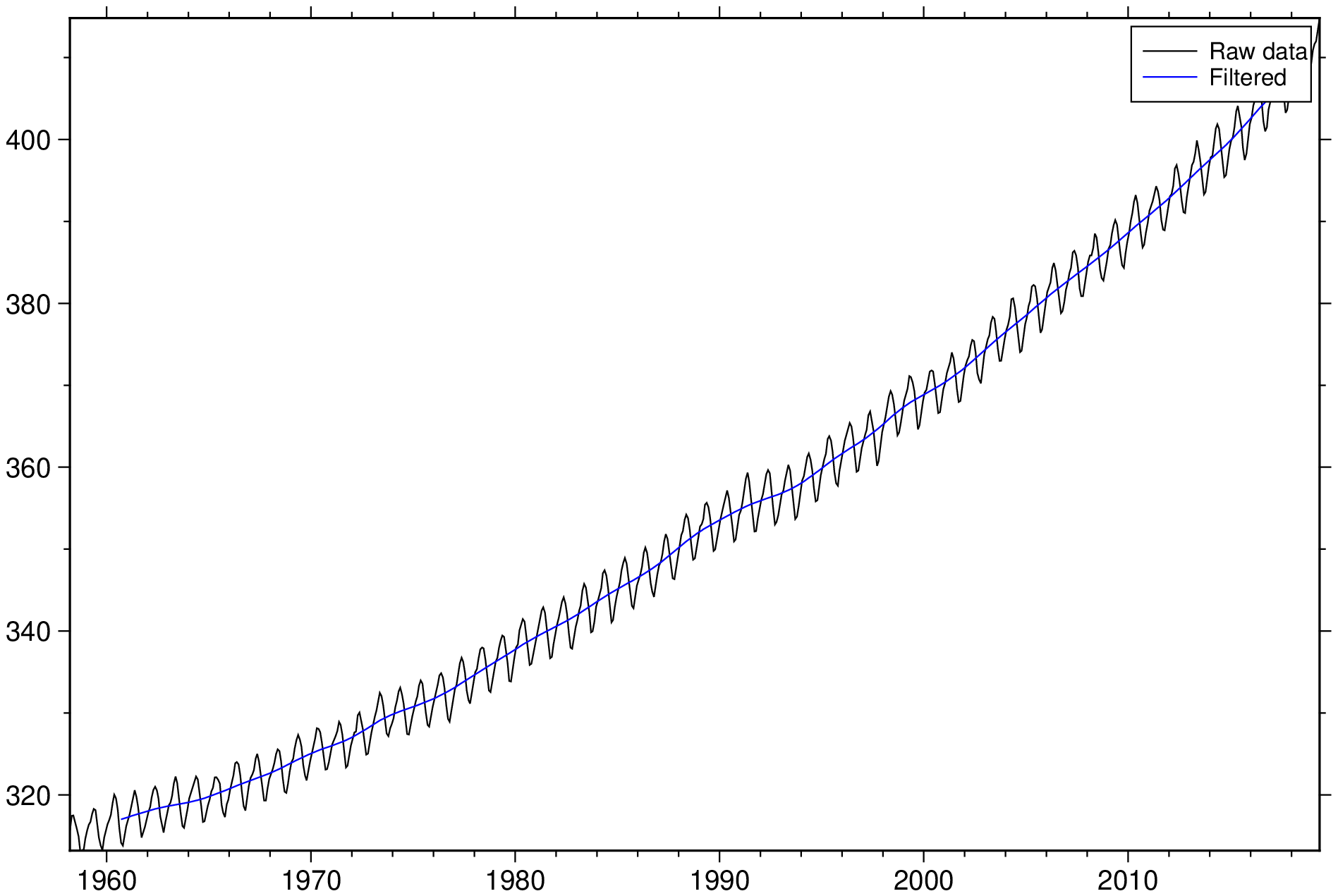
To filter the remote CO2 data set in the file MaunaLoa_CO2.txt (year, CO2) with a 5 year Gaussian filter, try

using GMT
D = filter1d("@MaunaLoa_CO2.txt", filter=(type=:gauss, width=5));
plot("@MaunaLoa_CO2.txt", legend="Raw data")
plot!(D, lc=:blue, legend="Filtered", show=1)

Data along track often have uneven sampling and gaps which we do not want to interpolate using sample1d. To find the median depth in a 50 km window every 25 km along the track of cruise v3312, stored in v3312.txt, checking for gaps of 10km and asymmetry of 0.3:

D = filter1d("v3312.txt", filter=(:Median,50), range=(0,100000,25), gap_width=10, symetry=0.3)

To smooth a noisy geospatial track using a Gaussian filter of full-width 100 km and not shorten the track, and add the distances to the file, use

D = filter1d("track.txt", range="k+a", ends=true, filter=(:gaussian, 200))

See Also

sample1d, gmtsplit