grd2cpt

grd2cpt(cmd0::String="", arg1=nothing, kwargs...)

keywords: GMT, Julia, histogram equalizetiond, colormaps

Make linear or histogram-equalized color palette table from grid

Description

grd2cpt reads one or more grid and computes a static color palette (CPT). Once computed the color palette stays as the current CPT until an image using it is finished, either with the show command or saved to file. The CPT is based on an existing dynamic master CPT of your choice, and the mapping from data value to colors is through the data's cumulative distribution function (CDF), so that the colors are histogram equalized. Thus if the grid(s) and the resulting CPT are used in grdimage with a linear projection, the colors will be uniformly distributed in area on the plot. Let z be the data values in the grid. Define CDF(Z) = (# of z < Z) / (# of z in grid). (NaNs are ignored). These z-values are then normalized to the master CPT and colors are sampled at the desired intervals.

The color palette includes three additional colors beyond the range of z-values. These are the background color (B) assigned to values lower than the lowest z-value, the foreground color (F) assigned to values higher than the highest z-value, and the NaN color (N) painted wherever values are undefined. For color tables beyond the current GMT offerings, visit cpt-city.

If the master CPT includes B, F, and N entries, these will be copied into the new master file. If not, the parameters COLOR_BACKGROUND, COLOR_FOREGROUND, and COLOR_NAN from the gmt.conf file or the command line will be used. This default behavior can be overruled using the options bg, overrule_bg or no_bg.

The color model (RGB, HSV or CMYK) of the palette created by makecpt will be the same as specified in the header of the master CPT. When there is no COLOR_MODEL entry in the master CPT, the COLOR_MODEL specified in the gmt.conf (see gmtset) file or on the command line will be used.

Required Arguments

ingrid : – A grid file name or a Grid type

Optional Arguments

• A or alpha or transparency : – alpha=xx | alpha="xx+a"
  Sets a constant level of transparency (0-100) for all color slices. Append +a to also affect the fore-, back-, and nan-colors.

• C or color or cmap or colormap or colorscale : – cmap=[[section/]master_cpt[+h[hinge]][+u|+Uunit]|local_cpt|color1,color2[,color3,...]]
  Name of an input CPT file. Generally, the input is one of the GMT master_cpt files (see Of Colors and Color Legends) and can be either addressed by master_cpt or section/master_cpt (without the .cpt extension). If given a master CPT with soft-hinges then you can enable the hinge at data value hinge via +h, whereas for hard-hinge CPTs you can adjust the location of the hinge. For any other master_cpt, you may convert their z-values from meter to another distance unit (append +Uunit) or from another unit to meter (append +uunit), with unit taken from e|f|k|M|n|u. One can also supply the file name of already custom made local_cpt file. Alternatively, give color1,color2[,color3,...] to build a linear continuous CPT from those colors automatically, where z starts at 0 and is incremented by one for each color. In this case colorn can be a r/g/b triplet, a color name, or an HTML hexadecimal color (e.g. #aabbcc). See also Setting color

• D or bg or background : – bg=true | bg=:i
  Select the back- and foreground colors to match the colors for lowest and highest z-values in the output CPT [Default uses the colors specified in the master file, or those defined by the parameters COLOR_BACKGROUND, COLOR_FOREGROUND, and COLOR_NAN]. Append i to match the colors for the lowest and highest values in the input (instead of the output) CPT.

• E or nlevels : – nlevels=true | nlevels=nlevels|"+c[+f<file>]"
  Create a linear color table by using the grid z-range as the new limits in the CPT, so the number of levels in the CPT remain unchanged. Alternatively, append nlevels and we will instead resample the color table into nlevels equidistant slices. As an option, append +c to estimate the cumulative density function of the data and assign color levels accordingly. If +c is used then you may optionally append +f<file> to save the CDF to file, or just use +c+f to return also a table with the CDF.

• F or color_model : – color_model=true|:r|:h|:c["+c"[label]]
  Force output CPT to be written with r/g/b codes, gray-scale values or color name (the default) or r/g/b codes only (r), or h-s-v codes (h), or c/m/y/k codes (c). Optionally or alternatively, append +c to write discrete palettes in categorical format. If label is appended then we create labels for each category to be used when the CPT is plotted. The label may be a comma-separated list of category names (you can skip a category by not giving a name), or give start[-], where we automatically build monotonically increasing labels from start (a single letter or an integer). Append - to build ranges start-start+1 instead. Note: If +cM is given and the number of categories is 12, then we automatically create a list of month names. Likewise, if +cD is given and the number of categories is 7 then we make a list of weekday names. The format of these labels will depend on the FORMAT_TIME_PRIMARY_MAP, GMT_LANGUAGE and possibly TIME_WEEK_START settings.

• G or truncate : – truncate=(zlo,zhi)
  Truncate the incoming CPT so that the lowest and highest z-levels are to zlo and zhi. If one of these equal NaN then we leave that end of the CPT alone. The truncation takes place before any resampling. See also Manipulating CPTs

• I or inverse or reverse : – inverse=true | inverse=:z
  Reverse the sense of color progression in the master CPT. Also exchanges the foreground and background colors, including those specified by the parameters COLOR_BACKGROUND and COLOR_FOREGROUND. Use inverse=:z to reverse the sign of z-values in the color table. Note that this change of z-direction happens before truncate and range values are used so the latter much be compatible with the changed z-range. See also Manipulating CPTs

• L or datarange or clim : – datarange=(minlimit, maxlimit)
  Limit range of CPT to (minlimit, maxlimit), and don't count data outside this range when estimating CDF(Z). To set only one limit, specify the other limit as "-" [Default uses min and max of data.]

• M or overrule_bg : – overrule_bg=true
  Overrule background, foreground, and NaN colors specified in the master CPT with the values of the parameters COLOR_BACKGROUND, COLOR_FOREGROUND, and COLOR_NAN specified in the gmt.conf file or on the command line. When combined with bg, only COLOR_NAN is considered.

• N or no_bg or nobg : – no_bg=true
  Make all the background, foreground, and NaN-color fields be white (since we can't remove them like in plain GMT).

• Q or log : – log=true | log=:i|:o
  Selects a logarithmic interpolation scheme [Default is linear]. log=:i expects input z-values to be log10(z), assigns colors, and writes out z [Default]. log=:o takes log10(z) first, assigns colors, and writes out z.

• R or region or limits : – limits=(xmin, xmax, ymin, ymax) | limits=(BB=(xmin, xmax, ymin, ymax),) | limits=(LLUR=(xmin, xmax, ymin, ymax),units="unit") | ...more
  Specify the region of interest. More at limits. For perspective view view, optionally add zmin,zmax. This option may be used to indicate the range used for the 3-D axes. You may ask for a larger w/e/s/n region to have more room between the image and the axes.

• S or symmetric : – symmetric=:h|l|m|u
  Force the color table to be symmetric about zero (from -R to +R). Append flag to set the range R: l for R =|zmin|, u for R = |zmax|, m for R = min(|zmin|, |zmax|), or h for R = max(|zmin|, |zmax|).

• T or range : – range=(min,max,inc) | range=n
  Set steps in CPT. Calculate entries in CPT from start to stop in steps of (inc). Default chooses arbitrary values by a crazy scheme based on equidistant values for a Gaussian CDF. Use range=n to select n points from such a cumulative normal distribution [11].

• V Verbose operation. This will write CDF(Z) estimates to stderr. [Default is silent.]

• W or categorical : – categorical=true | categorical=:w
  Do not interpolate the input color table but pick the output colors starting at the beginning of the color table, until colors for all intervals are assigned. This is particularly useful in combination with a categorical color table, like "categorical". Alternatively, use categorical=:w to produce a wrapped (cyclic) color table that endlessly repeats its range.

• Z or continuous : – continuous=true
  Force a continuous CPT [Default is discontinuous].

• name or save : – save="name.cpt"
  Save the color map with the save="name.cpt". When in modern mode this also automatically sets a required GMT option (-H).

• bo or binary_out : – binary_out=??
  Select native binary format for table output. More at

This option only applies if nlevels selects CDF output.

• h or header : – header=??
  Specify that input and/or output file(s) have n header records. More at

Notes on Transparency

The PostScript language originally had no accommodation for transparency. However, Adobe added an extension that allows developers to encode some forms of transparency using the PostScript language model but it is only realized when converting the PostScript to PDF (and via PDF to any raster image format). GMT uses this model but there are some limitations: Transparency can only be controlled on a per-object or per-layer basis. This means that a color specifications (such as those in CPTs of given via command-line options) only apply to vector graphic items (i.e., text, lines, polygon fills) or to an entire layer (which could include items such as PostScript images). This limitation rules out any mechanism of controlling transparency in such images on a pixel level.

Color Hinges

Some of the GMT master dynamic CPTs are actually two separate CPTs meeting at a hinge. Usually, colors may change dramatically across the hinge, which is used to separate two different domains (e.g., land and ocean across the shoreline, for instance). CPTs with a hinge will have their two parts stretched to the required range separately, i.e., the bottom part up to the hinge will be stretched independently of the part from the hinge to the top, according to the prescribed new range. Hinges are either hard or soft. Soft hinges must be activated by appending +h[hinge] to the CPT name. If the selected range does not include an activated soft or hard hinge then we only resample colors from the half of the CPT that pertains to the range. See Of Colors and Color Legends for more information.

Discrete versus Continuous CPT

All CPTs can be stretched, but only continuous CPTs can be sampled at new nodes (i.e., by given an increment in range). We impose this limitation to avoid aliasing the original CPT.

Examples

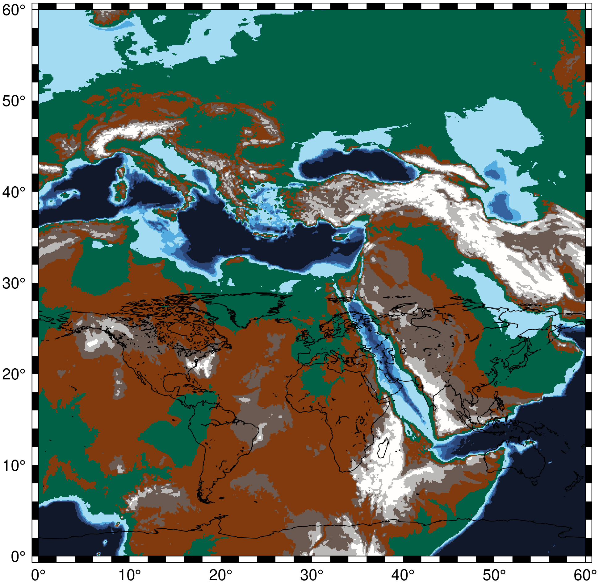
To get a reasonable and symmetrical color table for the data in the region 0/60/0/60 from the remote 5m relief file, using the geo color table, try:

using GMT
grd2cpt("@earth_relief_06m_g", region=(0,60,0,60), cmap=:geo, symetric=:u)
imshow("@earth_relief_06m_g", region=(0,60,0,60), coast=true)

Sometimes you don't want to make a CPT (yet) but would find it helpful to know that 90% of your data lie between z1 and z2, something you cannot learn from grdinfo. So you can do this to see some points on the CDF(Z) curve (use verbose=true option to see more):

grd2cpt("mydata.nc", verbose=true)

To make a CPT with entries from 0 to 200 in steps of 20, and ignore data below zero in computing CDF(Z), and use the built-in master cpt file relief, run

C = grd2cpt("mydata.nc", cmap=:relief, datarange=(0,10000), range=(0,200,20))

To determine the empirical cumulative density function of a grid and create a CPT that would give equal area to each color in the image, and return the CDF table as well, try:

using GMT
C, cdf = grd2cpt("@earth_relief_10m_g", nlevels="11+c+f");
imshow("@earth_relief_10m_g", cmap=C)

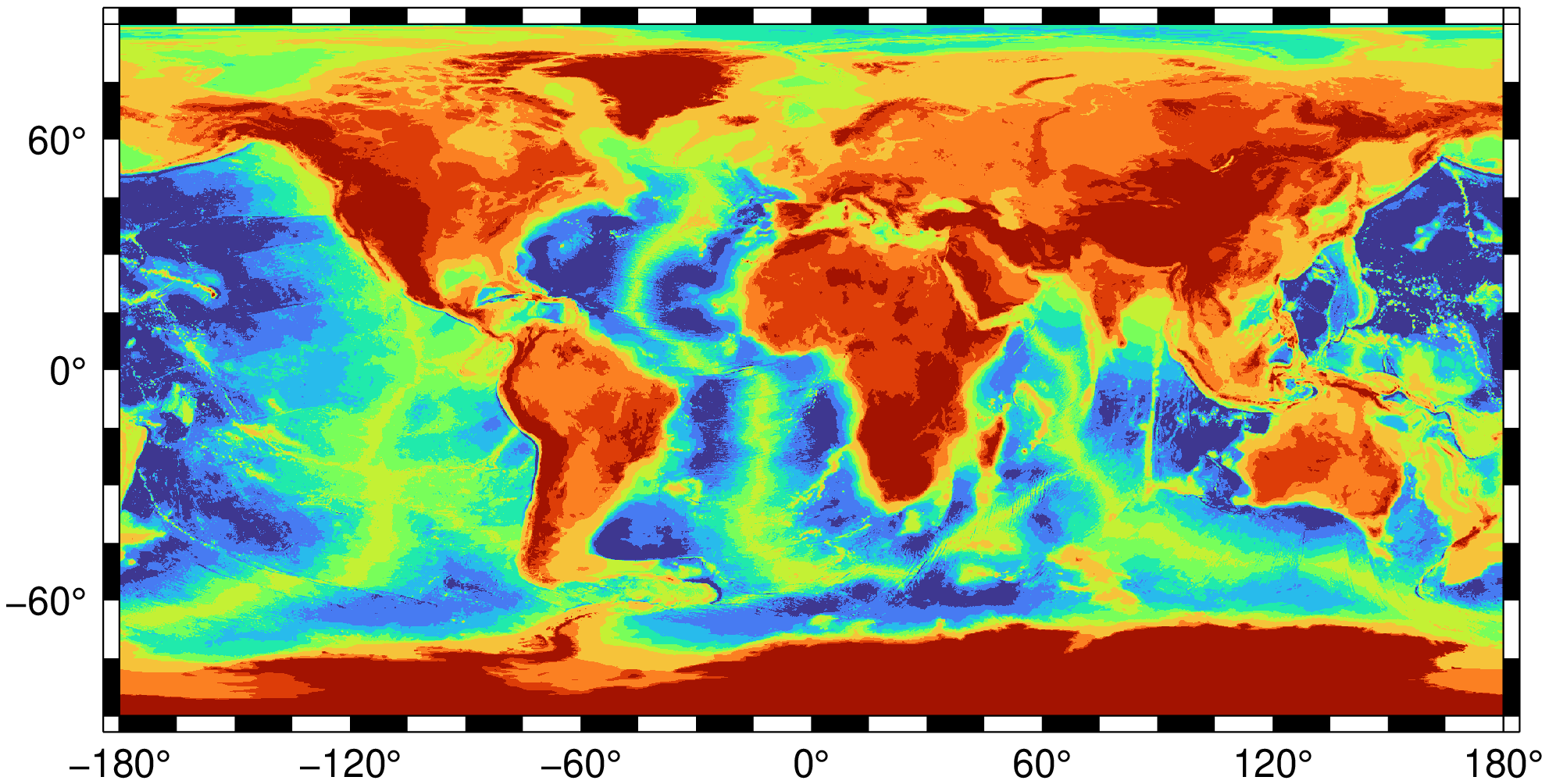
Here, cdf would be the cumulative hypsometric curve for the Earth.

See Also

grdhisteq, grdinfo, makecpt

References

Crameri, F., (2018). Scientific colour-maps. Zenodo. http://doi.org/10.5281/zenodo.1243862

Crameri, F. (2018), Geodynamic diagnostics, scientific visualisation and StagLab 3.0, Geosci. Model Dev., 11, 2541-2562, doi:10.5194/gmd-11-2541-2018.